Generalization in Classification
Dive into Deep Learning · §3.6
Generalization in Classification
How much should you trust a test score, and can we ever guarantee generalization before we see the data?
Memorizing is not learning
Why this matters
A sufficiently expressive model can memorize distinct training inputs and attain zero training error without defining useful predictions for new inputs.
The score we care about is the population error, on data we never trained on. Three questions stand between us and trusting it:
- How many test points estimate the error precisely?
- What if we reuse the same test set?
- Why expect a trained model to beat memorizing at all?
01
The Test Set
what a held-out score can, and cannot, tell you
Two errors: one we measure, one we want
The Test Set
On a fresh set \mathcal{D} of n points, the empirical error is the miss rate we can compute; the population error is the one we actually care about, over the whole distribution, which we never see:
\epsilon_\mathcal{D}(f) = \frac{1}{n}\sum_{i=1}^n \mathbf{1}\!\left(f(\mathbf{x}^{(i)}) \neq y^{(i)}\right) \qquad\text{vs.}\qquad \epsilon(f) = E_{(\mathbf{x},y)\sim P}\,\mathbf{1}\!\left(f(\mathbf{x}) \neq y\right).
For a fixed f, the test miss rate is just a sample mean of a \{0,1\} random variable: an unbiased estimate of \epsilon(f).
The square-root law of test error
The Test Set · convergence
The indicator \mathbf{1}(f(X)\neq Y) is Bernoulli. By the central limit theorem the test error concentrates on the true error, with standard deviation shrinking as \sigma/\sqrt{n}:
\epsilon_\mathcal{D}(f) \approx \epsilon(f) \pm \mathcal{O}(1/\sqrt{n}).
The \sqrt{n} rate implies that 2× the precision costs 4× the data; 10× the precision costs 100×. This rate is usually the best statistics can offer.
So how big a test set?
The Test Set · sample size
A Bernoulli variance is largest at error 0.5, so it is capped: \sigma^2=\epsilon(1-\epsilon)\le 0.25.
Want 95% confidence that \epsilon_\mathcal{D}(f) lands within \pm 0.01 of \epsilon(f)? Fit two standard deviations in that window:
2\sqrt{0.25/n}\le 0.01 \;\Longrightarrow\; n\approx 10{,}000.
Many benchmarks use test sets of this order. The uncertainty calculation is necessary when interpreting an improvement of 0.01.
Asymptotics vs. a bound valid at every finite n
The Test Set · finite samples
The \sqrt{n} law is asymptotic. Because the loss is bounded, Hoeffding’s inequality gives a guarantee that holds at any n:
P\!\left(|\epsilon_\mathcal{D}(f) - \epsilon(f)| \geq t\right) < 2\exp\!\left(-2nt^2\right).
Same target (\pm 0.01 at 95%), finite-sample answer valid at every n: n\approx 18{,}500 vs. the asymptotic 10{,}000. Guarantees that hold for every n are a bit more conservative, but in the same ballpark.
The √n law, simulated
The Test Set · convergence
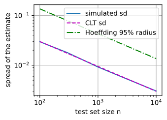
Fix a classifier with true error 0.1 and draw 1000 hypothetical test sets at each size n: the spread of the estimates marches down the predicted -\tfrac12 slope on log–log axes.
The simulated spread sits on the CLT line; the Hoeffding envelope runs parallel above it, the constant-factor price of a guarantee at every finite n.
02
Reusing the Test Set
multiple comparisons and adaptive overfitting
Reusing a test set for model selection
Test-Set Reuse
You evaluate model f_1 once, by the book, and report a confidence interval. You then develop f_2, tune it, and observe a better test score.
Now you reach for the final evaluation, and realize: you no longer have a test set. The data is still on disk, but it is no longer unseen.
Each test score used to guide development makes subsequent choices depend on the test set, weakening its independence as a final evaluation.
Two consequences of test-set reuse
Test-Set Reuse
False discovery. One classifier has a 5% chance of a misleading score. Test 20 of them and you have little power to rule out that one looks good by chance. This is multiple hypothesis testing.
Adaptive overfitting. f_2 was chosen after you saw f_1’s test score, so the choice depends on the test set. Once that information leaks to the modeler, it is no longer a true test set.
Selection alone raises the reported score
Test-Set Reuse
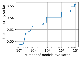
Evaluate k coin-flip classifiers (true accuracy exactly 0.5) on one shared test set of n = 1000 and track the best score so far: past 0.56 after ten thousand tries, by pure selection.
The climb grows like \sqrt{\log(k)/(2n)}, Hoeffding over k events at once. Best-of-many selection on a shared test set includes a selection effect of this kind.
Limit access to the test set
Test-Set Reuse · in practice
The worst-case theory motivates conservative test-set practice. In practice:
- Curate a real test set; consult it as rarely as possible.
- Correct confidence intervals for multiple comparisons.
- Be most careful when stakes are high and the set is small.
- Run rounds: demote each spent test set to a validation set.
03
Statistical Learning Theory
guaranteeing generalization a priori, from the model class alone
Uniform convergence over a model class
Learning Theory
A test set provides a post hoc estimate for one fitted model; it does not explain why a learning procedure generalizes. Learning theory wants a guarantee from the model class \mathcal{F} alone.
Under uniform convergence, with probability \ge 1-\delta, every f\in\mathcal{F} has its empirical error close to its true error at once. Then the selected empirical-risk minimizer inherits the uniform bound.
A single fixed f always generalizes. The danger is picking one out of many that got a lucky score.
The complexity trade-off
Learning Theory
Whether uniform convergence can hold depends entirely on how flexible \mathcal{F} is:
Memorizers are too flexible: zero training error, no generalization. Their training fit alone yields no useful uniform-convergence guarantee.
A single fixed f generalizes perfectly but fits nothing. Useful models live in between: flexible enough to fit, rigid enough to generalize.
Shattering: when can a line realize any labeling?
Learning Theory · VC dimension
A class shatters a set of points if it can realize every \pm labeling of them. A line in the plane shatters any 3 points, but no line realizes the XOR labeling of 4.
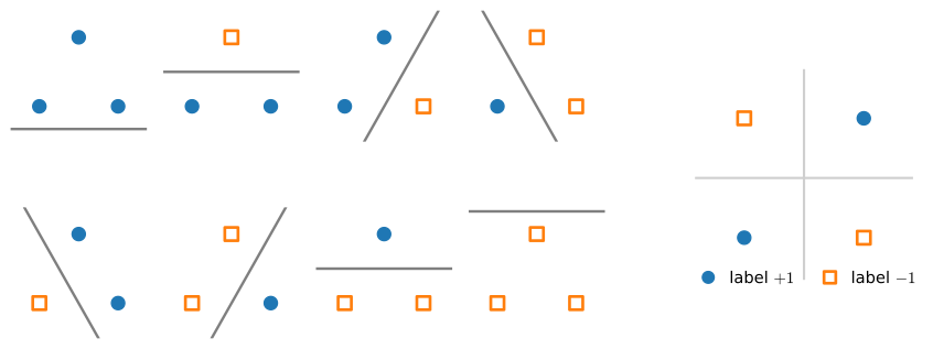
All 2^3=8 labelings of 3 points are linearly separable (left); the XOR labeling of 4 points is not (right). So plane lines shatter 3 points but not 4.
The VC dimension of linear models is d+1
Learning Theory · the bound
The VC dimension is the largest set a class can shatter. Lines in the plane: 3. Linear models in d dimensions: d+1, exactly.
- Lower bound: the points \{\mathbf{0}, \mathbf{e}_1, \ldots, \mathbf{e}_d\} are shattered by weights read off the desired labels (exercise 5).
- Upper bound: by Radon’s theorem any d+2 points split into two subsets with intersecting convex hulls, and no halfspace separates intersecting hulls.
Vapnik–Chervonenkis then bound the gap uniformly over the class:
\epsilon(f_\mathcal{S}) - \epsilon_\mathcal{S}(f_\mathcal{S}) < c\sqrt{\tfrac{\mathrm{VC}-\log\delta}{n}}
with probability \ge 1-\delta.
Fix the class and \delta: the familiar \mathcal{O}(1/\sqrt{n}) rate, now for the learned model.
Why this breaks for deep networks
Learning Theory · the paradox
VC dimension is exact for linear model classes, but the resulting generalization bounds for deep networks can be vacuous, requiring sample counts (perhaps trillions).
A deep net can fit random labels, so its VC dimension is enormous, yet it generalizes well on real data, and often better as it gets larger and deeper. These classical capacity bounds do not explain this empirical behavior.
The modern road, Rademacher complexity and the double-descent behavior of overparametrized models reproduced from scratch, is developed in the concentration-and-generalization section; the deep-learning story resumes in the generalization-in-deep-learning section.
Recap
Wrap-up
- Test set = an unbiased estimate of the true error; it converges at \mathcal{O}(1/\sqrt{n}). About 10k points give \pm 0.01 at 95%.
- Asymptotic vs finite: Hoeffding is valid at any n, and a little more conservative (~18.5k).
- Reuse affects validity: false discovery + adaptive overfitting. Treat a test set as scarce.
- Learning theory seeks a-priori guarantees via uniform convergence over a class \mathcal{F}.
- VC dimension = largest shatterable set; for linear models exactly d+1 (labels read off / Radon); it bounds the gap at \mathcal{O}(1/\sqrt{n}).
- Deep nets are not explained by these bounds, generalizing despite huge capacity: the puzzle of the generalization-in-deep-learning section, with the modern tools in the concentration-and-generalization section.