Environment and Distribution Shift
Dive into Deep Learning · §3.7
When deployment data differ from training data
Distribution shift: assumptions, consequences, and correction methods.
From prediction to deployment
Why this matters
We fit models to data and measure test accuracy. Deployment analysis must also ask where the data came from and how the prediction will be used.
A loan model finds that Oxfords repay, sneakers default. Approve everyone in Oxfords, and soon everyone wears Oxfords, with no change in who actually repays. The decision changed the relationship between footwear and repayment risk.
This is Goodhart’s law: when a measure becomes a target, it ceases to be a good measure. Deploying a model can perturb the very distribution it was trained on.
Train here, deploy there
The setup
Training data is drawn from a source distribution p_S(\mathbf{x}, y); at test time we meet a target p_T(\mathbf{x}, y) that may differ.
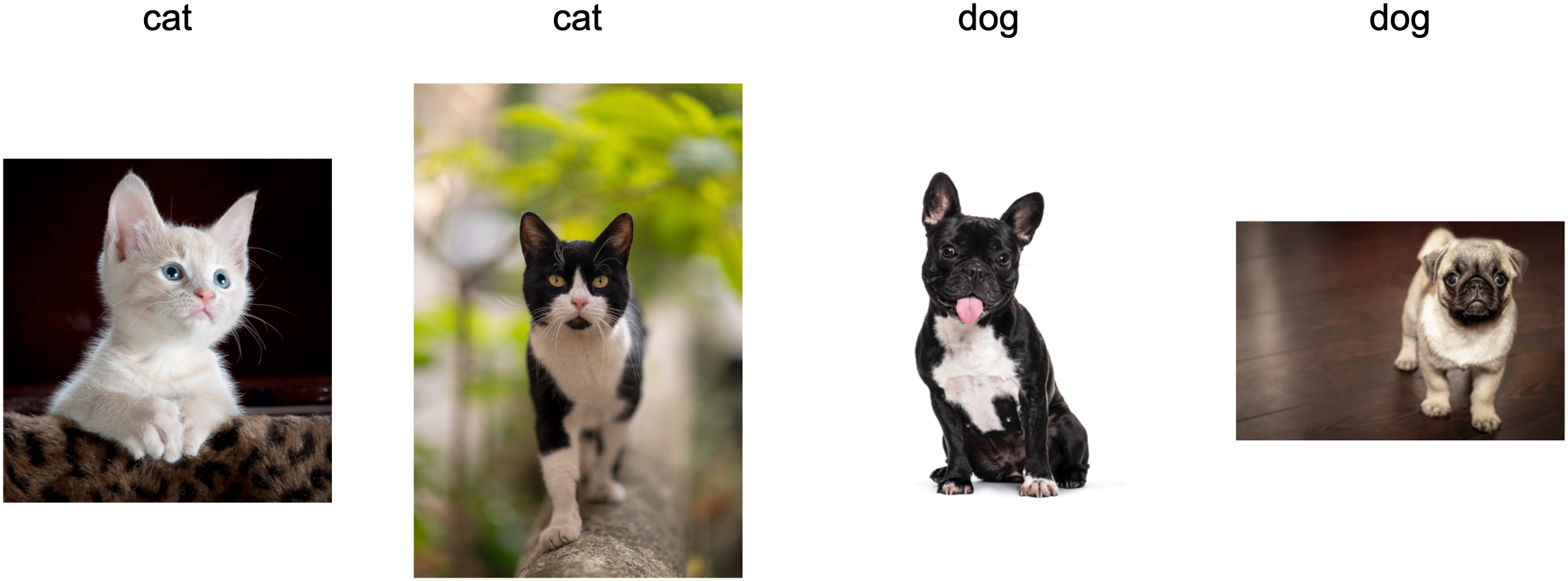
With no link between p_S and p_T, learning cannot transfer. Suppose the inputs are unchanged, p_S(\mathbf{x})=p_T(\mathbf{x}), but every label flips, p_S(y\mid\mathbf{x})=1-p_T(y\mid\mathbf{x}): “cats” become “dogs” overnight. No algorithm can tell this apart from no shift at all.
The way out is structure: assume how the world may change, and that assumption can enable detection or a specific correction.
01
Three Kinds of Shift
what stays fixed tells you what to do
Label shift: the mix moves
Three kinds of shift
The label frequencies P(y) change, but each class still looks the same: P(\mathbf{x}\mid y) is fixed.
The natural assumption when y causes \mathbf{x}: diseases cause symptoms, so as an outbreak shifts how common a diagnosis is, the symptom pattern per disease is unchanged.
Why prefer it when both could apply? Its corrections operate in label space, whose categories are typically far lower-dimensional than the input space.
Concept shift: the labels themselves move
Three kinds of shift
Now the definition of a label drifts: P(y\mid\mathbf{x}) changes because what counts as the answer changed.
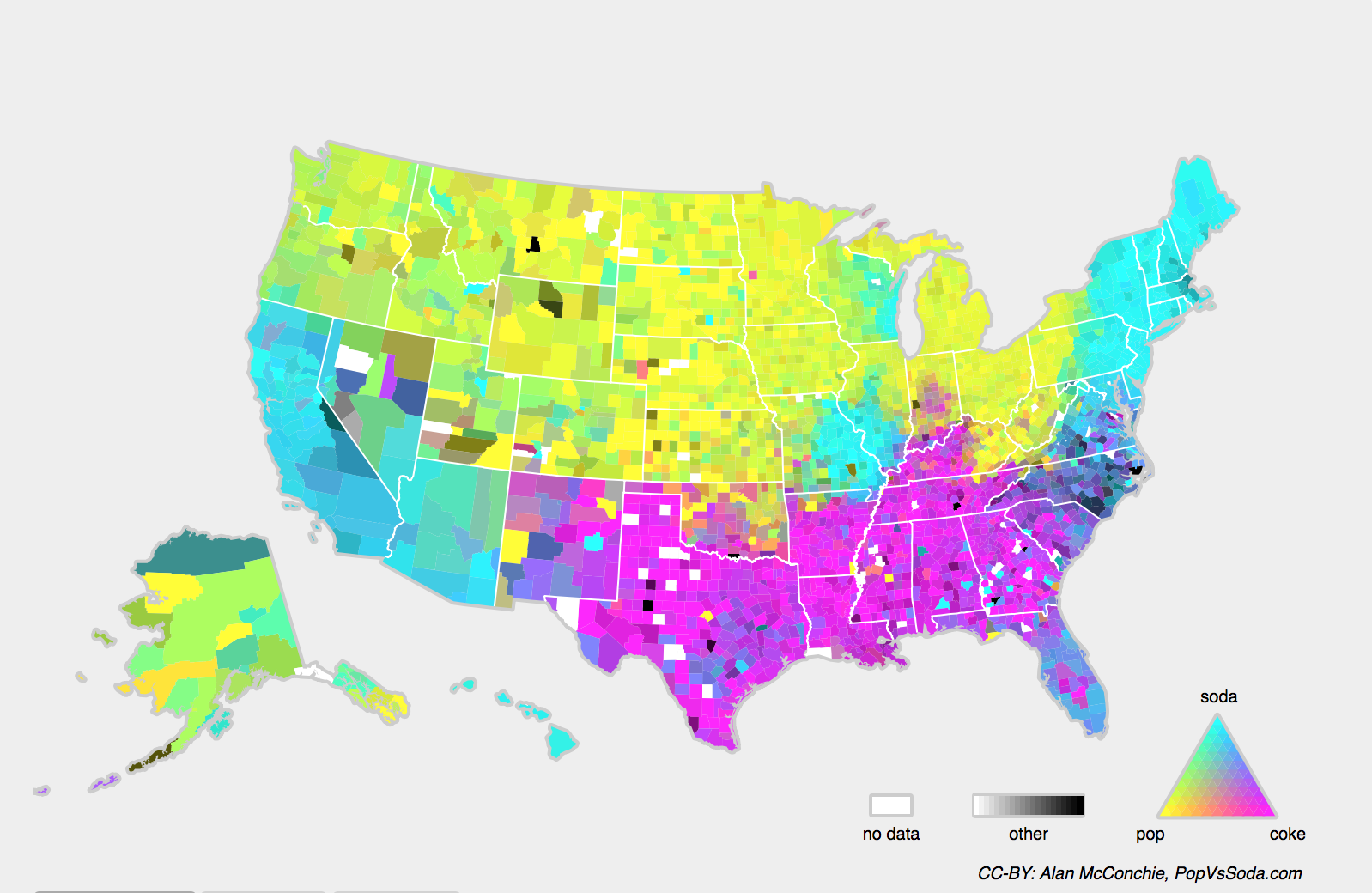
What people call a soft drink depends on where you ask (“soda”, “pop”, “coke”).
Diagnostic criteria, fashion, and job titles can drift this way across time or geography. Gradual drift can sometimes be tracked with fresh labeled data; abrupt changes require faster detection and may require a new model.
02
Consequences
spurious features and slow drift
The model learned the wrong thing
Spurious correlation
A blood-test startup drew healthy controls from students, sick patients from the clinic. The classifier hit near-perfect accuracy, on age, hormones, and diet, not the disease.
A tank-classification example. A network performs well on held-out images but fails in the field because tank photos were taken at noon and empty scenes at dawn. The model learned lighting, not the presence of a tank.
A model may rely on a feature correlated with the label in the sample but absent or changed at deployment.
Slow drift, stale model
Temporal drift
The subtler failure: the distribution moves gradually (a nonstationary world) and the model is never refreshed.
A spam filter stops working once spammers craft messages unlike any seen before.
A recommender keeps pushing Santa hats long after Christmas.
Performance can deteriorate gradually when the distribution changes and the model is not updated.
03
Correcting Shift
reweighting the risk we cannot see
Risk vs. empirical risk
The frame
What we want to minimize is the risk: expected loss under the true distribution p(\mathbf{x}, y).
R(f) = \mathbb{E}_{(\mathbf{x}, y)\sim p}\,[\,l(f(\mathbf{x}), y)\,].
We cannot evaluate it, so we minimize the empirical risk, the average loss on the training sample, and use it as an estimator under sampling assumptions.
\hat{R}(f) = \frac{1}{n}\sum_{i=1}^{n} l(f(\mathbf{x}_i), y_i).
Under shift, the training sample comes from the source distribution, so its empirical risk need not estimate target risk without a correction.
Reweight to the right distribution
Covariate shift correction
Labeled data comes from source q(\mathbf{x}), but we care about target p(\mathbf{x}). Under p(y\mid\mathbf{x})=q(y\mid\mathbf{x}), importance weighting rewrites target risk:
\mathbb{E}_{p}[\,l\,] = \mathbb{E}_{q}\!\left[\,\frac{p(\mathbf{x})}{q(\mathbf{x})}\, l\,\right].
So reweight each example by how much more likely it is under the target than the source, and minimize a weighted empirical risk:
\beta_i = \frac{p(\mathbf{x}_i)}{q(\mathbf{x}_i)}, \qquad \min_f\ \frac{1}{n}\sum_{i=1}^{n}\beta_i\, l(f(\mathbf{x}_i), y_i).
A classifier estimates the weights
Covariate shift correction
We do not know p/q. With equally weighted source and target domain samples, a classifier that distinguishes them (z=+1 for target, -1 for source) estimates odds equal to the density ratio:
\frac{P(z{=}1\mid\mathbf{x})}{P(z{=}{-}1\mid\mathbf{x})} = \frac{p(\mathbf{x})}{q(\mathbf{x})}.
With a logistic model P(z{=}1\mid\mathbf{x})=\sigma(h(\mathbf{x})) this collapses to \beta_i = \exp(h(\mathbf{x}_i)). We need only unlabeled target features \mathbf{x}\sim p.
Where the weights explode, and why we clip
Covariate shift correction · geometry
![]()
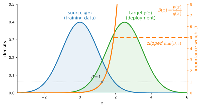
Training data comes from the source q (left curve); the risk we care about weights points by the target p (right curve). The weight \beta = p/q is near zero where only the source has mass, crosses 1 where the densities agree, and becomes large in the tail where the source has almost nothing; the dashed line clips it at a ceiling c.
Clip \beta_i \leftarrow \min(\exp(h(\mathbf{x}_i)), c): where the domains barely overlap, a few examples receive enormous weights and dominate the objective, so a little bias buys much less variance. If p > 0 where q = 0, the true weight is infinite: reweighting cannot recover support absent from the source sample.
The discriminator estimates the known ratio
Covariate shift correction · watch it work
A two-dimensional example uses source Gaussian at the origin, target the same Gaussian shifted to (2, 0), one shared curved labeling rule (covariate shift by construction), with a known answer: the true log-ratio is 2x_1 - 2. Pool the inputs, train the domain classifier h:
learned h(x) = 2.06 x1 +0.09 x2 -2.03 (true log-ratio: 2 x1 - 2)
beta on source data: mean 0.86, max 56.2
Learned: 2.06\,x_1 + 0.09\,x_2 - 2.03. The discriminator estimates the log density ratio, and note the \beta tail: one source point already carries weight 56.
Reweighting improves target accuracy in this example
Covariate shift correction · result
Train the actual classifier three ways on the same labeled source data; evaluate on the target, the domain we care about:
unweighted    target accuracy: 0.502   (source accuracy: 0.860)
weighted      target accuracy: 0.933   (source accuracy: 0.795)
clipped, c=5  target accuracy: 0.945   (source accuracy: 0.817)
Unweighted fits where the source lives: 0.502 on the target, near chance for this balanced binary task. Reweighting: 0.933, bought by a worse fit on the discounted source region, exactly the trade the identity prescribes. Clipping at c=5 limits the \beta > 50 outliers and even helps: 0.945.
Label shift: invert a confusion matrix
Label shift correction
Here P(y) shifts while P(\mathbf{x}\mid y) is fixed, so the weights are label ratios \beta_i=p(y_i)/q(y_i), and we never touch the high-dimensional inputs.
Take an off-the-shelf classifier, measure its k\times k confusion matrix \mathbf{C} on a source validation set (the very matrix we computed for Fashion-MNIST in the softmax-from-scratch section, column-normalized), and the average prediction \mu(\hat{\mathbf{y}}) on the (unlabeled) target. They are linked by total probability:
\mathbf{C}\, p(\mathbf{y}) = \mu(\hat{\mathbf{y}}) \quad\Longrightarrow\quad p(\mathbf{y}) = \mathbf{C}^{-1}\mu(\hat{\mathbf{y}}).
The system requires a nonsingular \mathbf{C}. Strict diagonal dominance (each diagonal entry exceeds the sum of the other entries in its row) is one sufficient condition; then form \beta_i and reweight.
Concept shift requires updating the model
Concept shift correction
Covariate reweighting cannot repair a changed P(y\mid\mathbf{x}); adaptation requires information about the new labeling relation.
When concept shift is gradual, as in changing ads or news, fresh labeled data can reveal the moving target. One practical response is:
Keep the current weights and take a few update steps on fresh data, rather than retraining from scratch. This allows the model to track gradual changes when the new sample is representative.
04
Beyond Passive Prediction
when the environment reacts to you
A taxonomy of learning problems
Learning settings
The preceding cases assumed passive prediction. The environment can also react:
- Batch: train once, deploy, never update (the smart catdoor).
- Online: data arrives one point at a time; predict, then learn from the outcome.
- Bandits: online, but a finite set of actions, so stronger guarantees.
- Control & RL: the environment remembers and responds, possibly adversarially (a thermostat, a chess opponent, other cars).
A strategy that is safe in a stationary world can fail once the world adapts to it, for example, an arbitrage opportunity may disappear after widespread use.
Predictions become decisions
Fairness & feedback
Deploying a model can automate decisions about people. Aggregate accuracy may be insufficient (the costs of different errors differ).
Predictive-policing feedback loop. More patrols → more crime recorded in that area → the model predicts even more crime there → still more patrols. The data feeds back into the model, reinforcing the allocation.
Watch for feedback loops, cost-sensitive errors, and whether you are solving the right problem at all.
Shift in the foundation-model era
Current benchmarks
Benchmarks like WILDS collect real shifts (hospitals, cameras, countries, time) along an axis orthogonal to our mechanism taxonomy:
Domain generalization: test domains never seen in training. Camelyon17: a tumor classifier trained on a few hospitals’ slides must survive a new hospital’s staining quirks.
Subpopulation shift: same domains, new proportions, so what matters is worst-group accuracy. CivilComments: average toxicity accuracy conceals much larger errors on some demographic groups.
OOD detection ≠ shift correction. Detection rejects inputs the model cannot handle; correction reweights for a target that is here to stay. A deployed system needs both, and a method that helps under one shift may fail under another, so evaluation must represent the deployment shift.
Summary
Wrap-up
- Shift = train and test distributions differ; unrecognized shift can cause deployment failures.
- Three kinds: covariate (P(\mathbf{x}) moves, \mathbf{x}\!\to\!y), label (P(y) moves, y\!\to\!\mathbf{x}), concept (the labels themselves move).
- Correct covariate shift by reweighting with \beta_i=p(\mathbf{x}_i)/q(\mathbf{x}_i), estimated by a source-vs-target classifier (demo: target accuracy 0.502 \to 0.933, clipped 0.945); label shift by inverting the confusion matrix.
- Beware the environment: it may remember your actions and feed them back. Measure on the shift you actually face (WILDS), and keep monitoring live systems.