Real Data Distribution

Generative Adversarial Networks

Generative Adversarial Networks

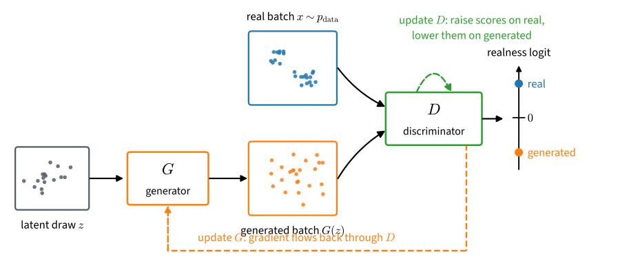
Generative Adversarial Networks (Goodfellow et al., 2014) — train a generator G and a discriminator D in a minimax game:

\min_G \max_D \; \mathbb{E}_{x \sim p_{\text{data}}} [\log D(x)] + \mathbb{E}_{z \sim p_z} [\log(1 - D(G(z)))].

• D tries to distinguish real samples from fake.
• G tries to produce samples that fool D.

At equilibrium, G’s distribution matches the data distribution. No likelihood, no MCMC — just two networks playing against each other.

The GAN architecture

Noise → generator → samples; discriminator vs real data.

This deck demos a tiny GAN on a 2D Gaussian. The next deck (DCGAN) generates real images.

Setup

Import backend utilities and define the plotting helper used to watch the 2D distribution during training:

%matplotlib inline
from d2l import torch as d2l
import torch
from torch import nn

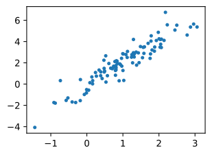
The “real” data is a 2D Gaussian, so success is visible: generated points should eventually match the same tilted elliptical cloud:

X = d2l.normal(0.0, 1, (1000, 2))
A = d2l.tensor([[1, 2], [-0.1, 0.5]])
b = d2l.tensor([1, 2])
data = d2l.matmul(X, A) + b

Sampling Real Batches

Training batches are iid draws from the target Gaussian. The discriminator only sees samples, not the analytic density:

d2l.set_figsize()
d2l.plt.scatter(d2l.numpy(data[:100, 0]), d2l.numpy(data[:100, 1]));
print(f'The covariance matrix is\n{d2l.matmul(A.T, A)}')

The covariance matrix is
tensor([[1.0100, 1.9500],
        [1.9500, 4.2500]])

Inspecting Real Samples

The scatter plot is the visual target for the generator. Later training plots should move the generated samples toward this shape:

batch_size = 8
data_iter = d2l.load_array((data,), batch_size)

Generator

Tiny MLP: latent z → 2D output. Maps the prior distribution to (hopefully) the data distribution:

net_G = nn.Sequential(nn.Linear(2, 2))

Discriminator

Tiny MLP, sigmoid output: 2D point → P(real). Standard binary classifier:

net_D = nn.Sequential(
    nn.Linear(2, 5), nn.Tanh(),
    nn.Linear(5, 3), nn.Tanh(),
    nn.Linear(3, 1))

Discriminator Update

For each batch:

1. Sample fake G(z), real x. Update D on \log D(x) + \log(1 - D(G(z))).

def update_D(X, Z, net_D, net_G, loss, trainer_D):
    """Update discriminator."""
    batch_size = X.shape[0]
    ones = torch.ones((batch_size,), device=X.device)
    zeros = torch.zeros((batch_size,), device=X.device)
    trainer_D.zero_grad()
    real_Y = net_D(X)
    fake_X = net_G(Z)
    # Do not need to compute gradient for `net_G`, detach it from
    # computing gradients.
    fake_Y = net_D(fake_X.detach())
    loss_D = (loss(real_Y, ones.reshape(real_Y.shape)) +
              loss(fake_Y, zeros.reshape(fake_Y.shape))) / 2
    loss_D.backward()
    trainer_D.step()
    return loss_D

Generator Update

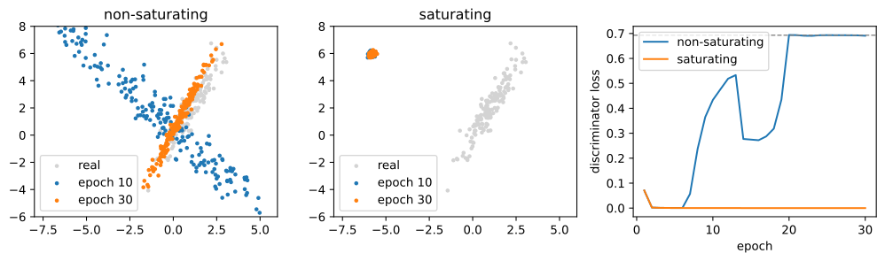
Sample fresh fakes; update G on \log D(G(z)) (the “non-saturating” form). It gives stronger gradients early in training than directly minimizing \log(1-D(G(z))):

def update_G(Z, net_D, net_G, loss, trainer_G):
    """Update generator."""
    batch_size = Z.shape[0]
    ones = torch.ones((batch_size,), device=Z.device)
    trainer_G.zero_grad()
    # We could reuse `fake_X` from `update_D` to save computation
    fake_X = net_G(Z)
    # Recomputing `fake_Y` is needed since `net_D` is changed
    fake_Y = net_D(fake_X)
    loss_G = loss(fake_Y, ones.reshape(fake_Y.shape))
    loss_G.backward()
    trainer_G.step()
    return loss_G

Training loop

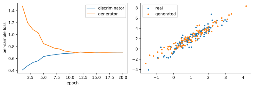
Alternate one discriminator step and one generator step. The losses are useful diagnostics, but the sample plot is the clearest signal that the generator distribution is moving in the right direction:

def train(net_D, net_G, data_iter, num_epochs, lr_D, lr_G, latent_dim, data):
    loss = nn.BCEWithLogitsLoss(reduction='sum')
    for w in net_D.parameters():
        nn.init.normal_(w, 0, 0.02)
    for w in net_G.parameters():
        nn.init.normal_(w, 0, 0.02)
    trainer_D = torch.optim.Adam(net_D.parameters(), lr=lr_D)
    trainer_G = torch.optim.Adam(net_G.parameters(), lr=lr_G)
    animator = d2l.Animator(xlabel='epoch', ylabel='loss',
                            xlim=[1, num_epochs], nrows=2, figsize=(5, 5),
                            legend=['discriminator', 'generator'])
    animator.fig.subplots_adjust(hspace=0.3)
    for epoch in range(num_epochs):
        # Train one epoch
        timer = d2l.Timer()
        metric = d2l.Accumulator(3)  # loss_D, loss_G, num_examples
        for (X,) in data_iter:
            batch_size = X.shape[0]
            Z = torch.normal(0, 1, size=(batch_size, latent_dim))
            metric.add(update_D(X, Z, net_D, net_G, loss, trainer_D),
                       update_G(Z, net_D, net_G, loss, trainer_G),
                       batch_size)
        # Visualize generated examples
        Z = torch.normal(0, 1, size=(100, latent_dim))
        fake_X = net_G(Z).detach().numpy()
        animator.axes[1].cla()
        animator.axes[1].scatter(data[:, 0], data[:, 1])
        animator.axes[1].scatter(fake_X[:, 0], fake_X[:, 1])
        animator.axes[1].legend(['real', 'generated'])
        # Show the losses
        loss_D, loss_G = metric[0]/metric[2], metric[1]/metric[2]
        animator.add(epoch + 1, (loss_D, loss_G))
    print(f'loss_D {loss_D:.3f}, loss_G {loss_G:.3f}, '
          f'{metric[2] / timer.stop():.1f} examples/sec')

Training Run

The final generated cloud should overlap the target Gaussian. If all samples collapse to a small region, the generator has found a mode-collapse failure instead of matching the distribution:

lr_D, lr_G, latent_dim, num_epochs = 0.05, 0.005, 2, 20
train(net_D, net_G, data_iter, num_epochs, lr_D, lr_G,
      latent_dim, d2l.numpy(data[:100]))

loss_D 0.693, loss_G 0.693, 2786.9 examples/sec

Recap

• GAN = generator + discriminator playing a minimax game.
• Equilibrium: G’s distribution = data distribution, D’s output is 1/2 everywhere.
• Notoriously tricky to train: mode collapse, vanishing gradients early on, training instability.
• Modern variants (WGAN, WGAN-GP, StyleGAN, BigGAN) fix pieces of this; the core minimax idea stays.