GP regression has a closed-form posterior. Given training data (\mathbf{X}, \mathbf{y}) and noise \sigma_n^2, the posterior at a new test point \mathbf{x}_* is Gaussian with:
Mean = best linear unbiased estimate. Variance = calibrated uncertainty. Both fall out of multivariate- Gaussian conditioning.
Hyperparameters (length-scale, noise, signal variance) are learned by maximizing the log marginal likelihood — Bayesian Occam’s razor in closed form.
The posterior equations
from d2l import torch as d2limport numpy as npfrom scipy.spatial import distance_matrixfrom scipy import optimizeimport matplotlib.pyplot as pltimport mathimport torchimport gpytorchimport os# Seed RNGs so the from-scratch fit and the GPyTorch optimization land# at reproducible values for the prose numbers below.np.random.seed(2)torch.manual_seed(2)d2l.set_figsize()
From-Scratch Setup
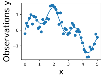
Build the training and test inputs, choose a kernel, and prepare the covariance matrices used by the GP posterior:
The predictive mean and covariance are Gaussian-conditioning formulae. Implement them with linear solves rather than explicit matrix inverses when scaling this beyond a toy example:
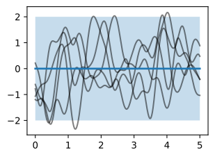
mean = np.zeros(test_x.shape[0])cov = d2l.rbfkernel(test_x, test_x, ls=0.2)
Learning Kernel Hyperparameters
Maximize log marginal likelihood to fit the length-scale, signal variance, and observation noise. The output should move toward a smooth fit without driving noise to zero:
prior_samples = np.random.multivariate_normal(mean=mean, cov=cov, size=5)d2l.plt.plot(test_x, prior_samples.T, color='black', alpha=0.5)d2l.plt.plot(test_x, mean, linewidth=2.)d2l.plt.fill_between(test_x, mean -2* np.sqrt(np.diag(cov)), mean +2* np.sqrt(np.diag(cov)), alpha=0.25)d2l.plt.show()
Visualizing predictions
Mean prediction + 2σ shaded band — uncertainty grows between training points and at the edges of the data:
ell_est =0.4post_sig_est =0.5def neg_MLL(pars): K = d2l.rbfkernel(train_x, train_x, ls=pars[0])# Solve (K + sigma^2 I) z = y rather than inverting the matrix; this is# numerically more stable and a bit cheaper. A = K + pars[1] **2* np.eye(train_x.shape[0]) alpha = np.linalg.solve(A, train_y) kernel_term =-0.5* train_y @ alpha sign, logabsdet = np.linalg.slogdet(A) logdet =-0.5* logabsdet const =-train_x.shape[0] /2.* np.log(2* np.pi)return-(kernel_term + logdet + const)learned_hypers = optimize.minimize(neg_MLL, x0=np.array([ell_est,post_sig_est]), bounds=((0.01, 10.), (0.01, 10.)))ell = learned_hypers.x[0]post_sig_est = learned_hypers.x[1]
Latent-function uncertainty
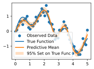
The shaded region below is a credible set for the noise-free latent function, not for future noisy observations. It should contain the true function, but it should not be expected to contain every data point:
K_x_xstar = d2l.rbfkernel(train_x, test_x, ls=ell)K_x_x = d2l.rbfkernel(train_x, train_x, ls=ell)K_xstar_xstar = d2l.rbfkernel(test_x, test_x, ls=ell)# Solve against (K_x_x + sigma^2 I) once rather than inverting the matrix:# `np.linalg.solve` is numerically more stable and a bit cheaper.A = K_x_x + post_sig_est **2* np.eye(train_x.shape[0])post_mean = K_x_xstar.T @ np.linalg.solve(A, train_y)post_cov = K_xstar_xstar - K_x_xstar.T @ np.linalg.solve(A, K_x_xstar)lw_bd = post_mean -2* np.sqrt(np.diag(post_cov))up_bd = post_mean +2* np.sqrt(np.diag(post_cov))d2l.plt.scatter(train_x, train_y)d2l.plt.plot(test_x, test_y, linewidth=2.)d2l.plt.plot(test_x, post_mean, linewidth=2.)d2l.plt.fill_between(test_x, lw_bd, up_bd, alpha=0.25)d2l.plt.legend(['Observed Data', 'True Function', 'Predictive Mean', '95% Set on True Func'])d2l.plt.show()
Two kinds of uncertainty
For noisy observations, uncertainty has two components:
Epistemic: reducible uncertainty about the latent function, captured by diag(post_cov).
Aleatoric: irreducible observation noise, captured by post_sig_est**2.
Same model, library implementation. Handles batched inference, GPU, and the linear-algebra abstractions used by larger GP models:
# First let's convert our data into tensors for use with PyTorchtrain_x = torch.from_numpy(np.asarray(train_x)).float()train_y = torch.from_numpy(np.asarray(train_y)).float()test_y = torch.from_numpy(np.asarray(test_y)).float()# We are using exact GP inference with a zero mean and RBF kernelclass ExactGPModel(gpytorch.models.ExactGP):def__init__(self, train_x, train_y, likelihood):super(ExactGPModel, self).__init__(train_x, train_y, likelihood)self.mean_module = gpytorch.means.ZeroMean()self.covar_module = gpytorch.kernels.ScaleKernel( gpytorch.kernels.RBFKernel())def forward(self, x): mean_x =self.mean_module(x) covar_x =self.covar_module(x)return gpytorch.distributions.MultivariateNormal(mean_x, covar_x)
GPyTorch Training Objective
The Gaussian likelihood contributes the noise parameter; the negative marginal log likelihood is the training loss for kernel hyperparameters:
# Initialize Gaussian likelihoodlikelihood = gpytorch.likelihoods.GaussianLikelihood()model = ExactGPModel(train_x, train_y, likelihood)training_iter =50# Find optimal model hyperparametersmodel.train()likelihood.train()# Use the adam optimizer, includes GaussianLikelihood parametersoptimizer = torch.optim.Adam(model.parameters(), lr=0.1) # Set our loss as the negative log GP marginal likelihoodmll = gpytorch.mlls.ExactMarginalLogLikelihood(likelihood, model)
Optimizing GP Hyperparameters
The printed length-scale and noise values should settle as the marginal likelihood improves. This is full-batch optimization, not minibatch SGD over independent examples:
for i inrange(training_iter):# Zero gradients from previous iteration optimizer.zero_grad()# Output from model output = model(train_x)# Calc loss and backprop gradients loss =-mll(output, train_y) loss.backward()if i %10==0:print(f'Iter {i+1:d}/{training_iter:d} - Loss: {loss.item():.3f} 'f'squared lengthscale: 'f'{model.covar_module.base_kernel.lengthscale.item():.3f} 'f'noise variance: {model.likelihood.noise.item():.3f}') optimizer.step()
Exact GP regression needs the matrix \mathbf{K}+\sigma_n^2\mathbf{I}.
Training log marginal likelihood uses a Cholesky factorization: \mathcal{O}(n^3) time and \mathcal{O}(n^2) memory.
Predictive means require triangular solves; predictive variances are usually more expensive than means.
The bottleneck is linear algebra, not evaluating the kernel.
Scalable GPs change the algebra: inducing points, structured kernels/KISS-GP, conjugate gradients, and variational objectives. Their complexity depends on assumptions such as number of inducing points, grid structure, and solver tolerance; it is not generically linear in n.
GPyTorch (cont.)
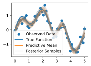
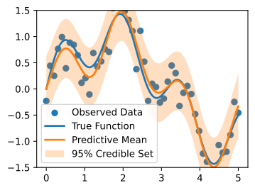
Switch to evaluation mode to compute the predictive posterior, then plot the mean and 95% credible set in observation space:
# Get into evaluation (predictive posterior) modetest_x = torch.from_numpy(np.asarray(test_x)).float()model.eval()likelihood.eval()observed_pred = likelihood(model(test_x))
with torch.no_grad():# Initialize plot f, ax = d2l.plt.subplots(1, 1, figsize=(4, 3))# Get upper and lower bounds for 95\% credible set (in this case, in# observation space) lower, upper = observed_pred.confidence_region() ax.scatter(train_x.numpy(), train_y.numpy()) ax.plot(test_x.numpy(), test_y.numpy(), linewidth=2.) ax.plot(test_x.numpy(), observed_pred.mean.numpy(), linewidth=2.) ax.fill_between(test_x.numpy(), lower.numpy(), upper.numpy(), alpha=0.25) ax.set_ylim([-1.5, 1.5]) ax.legend(['Observed Data', 'True Function', 'Predictive Mean', '95% Credible Set'])
Recap
GP regression posterior is closed-form Gaussian; mean + variance fall out of conjugate updates.
Hyperparameters fit by maximizing the log marginal likelihood — automatic capacity control.
Exact training cost is cubic from Cholesky factorization; scalable approximations trade exactness for structured or iterative linear algebra.
Workhorse for Bayesian optimization, active learning, and uncertainty-aware regression.