Denoising Score Matching

Dive into Deep Learning · §17.4

Denoising score matching
perturb the data · regress onto the conditional score · Tweedie’s formula · noise as a bias–variance knob

Three Problems, One Device: Add Noise

the Jacobian trace costs a derivative pass per dimension;
the score is unconstrained where the data are absent;
image data concentrate on or near a low-dimensional set, where the score is undefined or ill-conditioned.

\tilde{\mathbf{x}} = \mathbf{x} + \sigma \boldsymbol{\epsilon}, \qquad p_\sigma = p * \mathcal{N}(\mathbf{0}, \sigma^2 I)

p_\sigma is positive and smooth everywhere, and it approaches the data distribution as \sigma \to 0.

The Conditional Score Is a Gaussian Computation

\nabla_{\tilde{\mathbf{x}}} \log p_\sigma(\tilde{\mathbf{x}} \mid \mathbf{x}) = \frac{\mathbf{x} - \tilde{\mathbf{x}}}{\sigma^2} = -\frac{\boldsymbol{\epsilon}}{\sigma}

J_{\textrm{DSM}}(\boldsymbol{\theta}) = \tfrac{1}{2}\, \mathbb{E}_{\mathbf{x},\, \tilde{\mathbf{x}}} \Big\| \mathbf{s}_{\boldsymbol{\theta}}(\tilde{\mathbf{x}}) - \frac{\mathbf{x} - \tilde{\mathbf{x}}}{\sigma^2} \Big\|^2

Draw a point, add noise, regress onto the vector that points back. No Jacobian.

Vincent’s Theorem: Regression to the Conditional Mean

Least squares recovers \mathbb{E}[Y \mid X], and

\mathbb{E}\!\left[ \frac{\mathbf{x} - \tilde{\mathbf{x}}}{\sigma^2} \,\Big|\, \tilde{\mathbf{x}} \right] = \nabla_{\tilde{\mathbf{x}}} \log p_\sigma(\tilde{\mathbf{x}})

so J_{\textrm{DSM}} equals the Fisher divergence to p_\sigma plus a constant;
the model learns the score of the perturbed data;
the loss floor is half the average posterior variance of the target, not zero.

Tweedie’s Formula: the Score Is a Denoiser

\mathbb{E}[\mathbf{x} \mid \tilde{\mathbf{x}}] = \tilde{\mathbf{x}} + \sigma^2\, \nabla_{\tilde{\mathbf{x}}} \log p_\sigma(\tilde{\mathbf{x}})

the minimum-mean-squared-error denoiser moves along the score by \sigma^2;
noise prediction: \mathbf{s}_{\boldsymbol{\theta}} = -\boldsymbol{\epsilon}_{\boldsymbol{\theta}} / \sigma gives a unit-variance regression target.

The Noise Level Trades Bias against Variance

torch.manual_seed(0)
mix = d2l.GaussianMixture(means=[[-2.5, -1.5], [2.5, -1.5], [0.0, 2.5]],
                          weights=[0.5, 0.3, 0.2], std=0.5)
data, test = mix.sample(2000), mix.sample(2000)

def denoising_loss(score, x, sigma):
    eps = torch.randn_like(x)
    return 0.5 * ((score(x + sigma * eps) + eps / sigma) ** 2).sum(1).mean()

def fisher_divergence(score, x, sigma=0.0):
    """0.5 E||s(x) - grad log p_sigma(x)||^2 on the given points."""
    with torch.no_grad():
        return 0.5 * ((score(x) - mix.score(x, sigma=sigma)) ** 2).sum(1).mean().item()

def train(loss_fn, steps=2000, lr=1e-3, seed=1):
    torch.manual_seed(seed)
    score = d2l.ScoreNet()
    optimizer = torch.optim.Adam(score.parameters(), lr=lr)
    for step in range(steps):
        x = data[torch.randint(0, len(data), (256,))]
        loss = loss_fn(score, x)
        optimizer.zero_grad(), loss.backward(), optimizer.step()
    return score

scores = {}
print(f'{"sigma":>5} {"vs. score of p_sigma":>21} {"vs. score of the data":>22}')
for sigma in (0.1, 0.3, 1.0):
    scores[sigma] = train(lambda s, x: denoising_loss(s, x, sigma))
    noisy_test = test + sigma * torch.randn_like(test)
    print(f'{sigma:>5} {fisher_divergence(scores[sigma], noisy_test, sigma):>21.3f} '
          f'{fisher_divergence(scores[sigma], test):>22.3f}')

sigma  vs. score of p_sigma  vs. score of the data
  0.1                 0.269                  0.286
  0.3                 0.093                  0.375
  1.0                 0.006                  2.674

From \sigma = 0.1 to \sigma = 1: a much better fit to the perturbed score, a much worse match to the data score. No single level gives both.

Coverage Grows with the Noise

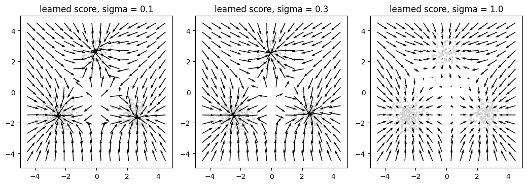
At \sigma = 1 the field is organized everywhere the noisy points reached, including between the modes.

A Score of Fashion-MNIST in a Minute

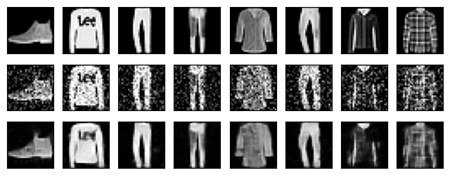
per-pixel squared error: noisy 0.251, denoised 0.031

Trained only to predict the noise; Tweedie’s formula turns the prediction into a reconstruction. The output estimates a posterior mean, hence smooth.

Recap

Perturb with \mathcal{N}(\mathbf{0}, \sigma^2 I); the conditional score is -\boldsymbol{\epsilon} / \sigma.
Denoising score matching regresses onto it and, by Vincent’s theorem, learns \nabla \log p_\sigma with no Jacobian.
Tweedie: score \Leftrightarrow optimal denoiser.
\sigma trades bias for variance and coverage. Next: sampling from a learned score, and where a single \sigma fails.