torch.manual_seed(0)
mix = d2l.GaussianMixture(means=[[-2.5, -1.5], [2.5, -1.5], [0.0, 2.5]],
                          weights=[0.5, 0.3, 0.2], std=0.5)
data, test = mix.sample(2000), mix.sample(2000)

T = 200
beta = torch.linspace(1e-4, 0.1, T)
alpha = 1 - beta
alpha_bar = torch.cumprod(alpha, 0)
print(f'alpha_bar_T = {alpha_bar[-1]:.1e}: after T steps the data are scaled '
      f'by {alpha_bar[-1].sqrt():.3f}')

torch.manual_seed(1)
x = data.clone()
for t in range(T):  # the chain, step by step
    x = alpha[t].sqrt() * x + beta[t].sqrt() * torch.randn_like(x)
    if t + 1 in (10, 50, 200):
        one_shot = (alpha_bar[t].sqrt() * data
                    + (1 - alpha_bar[t]).sqrt() * torch.randn_like(data))
        print(f'step {t + 1:3d}: chain: mean {[round(m, 3) for m in x.mean(0).tolist()]}, '
              f'var {x.var(0).mean():.3f} | one shot: mean '
              f'{[round(m, 3) for m in one_shot.mean(0).tolist()]}, '
f'var {one_shot.var(0).mean():.3f}')Denoising Diffusion Probabilistic Models
Dive into Deep Learning · §17.7
Denoising diffusion probabilistic models
a fixed forward chain · a learned reverse chain · a variational bound that becomes noise prediction
The Forward Process Turns Data into Noise in T Steps
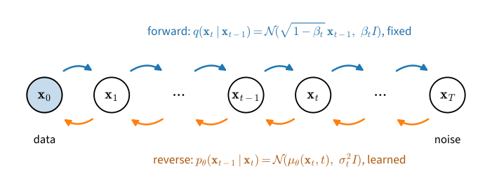
q(\mathbf{x}_t \mid \mathbf{x}_{t-1}) = \mathcal{N}\big(\sqrt{1 - \beta_t}\, \mathbf{x}_{t-1},\ \beta_t I\big), \qquad q(\mathbf{x}_t \mid \mathbf{x}_0) = \mathcal{N}\big(\sqrt{\bar{\alpha}_t}\, \mathbf{x}_0,\ (1 - \bar{\alpha}_t) I\big)
Variance preserving: the chain ends close to a standard Gaussian, whatever the data scale, once \sqrt{\bar{\alpha}_T}\, \mathbf{x}_0 is negligible.
The Closed-Form Marginal, Checked by Simulation
alpha_bar_T = 3.2e-05: after T steps the data are scaled by 0.006
step  10: chain: mean [-0.454, -0.76], var 3.838 | one shot: mean [-0.457, -0.766], var 3.838
step  50: chain: mean [-0.338, -0.563], var 2.554 | one shot: mean [-0.344, -0.553], var 2.554
step 200: chain: mean [-0.036, -0.021], var 0.990 | one shot: mean [-0.003, 0.001], var 0.966
Any step is one Gaussian draw from the data; training never simulates the chain.
The Reverse Process Is a Latent-Variable Model
p_{\boldsymbol{\theta}}(\mathbf{x}_{0:T}) = p(\mathbf{x}_T) \prod_{t=1}^{T} p_{\boldsymbol{\theta}}(\mathbf{x}_{t-1} \mid \mathbf{x}_t), \qquad p_{\boldsymbol{\theta}}(\mathbf{x}_{t-1} \mid \mathbf{x}_t) = \mathcal{N}\big(\boldsymbol{\mu}_{\boldsymbol{\theta}}(\mathbf{x}_t, t),\ \sigma_t^2 I\big)
- small steps: the reversal of a Gaussian step is nearly Gaussian;
- \mathbf{x}_{1:T} are latents; the likelihood of \mathbf{x}_0 is an intractable integral;
- so bound it, with the forward process as the auxiliary distribution.
The Bound Splits into One Term per Step
L_{\textrm{VLB}} = \underbrace{\mathrm{KL}\big(q(\mathbf{x}_T \mid \mathbf{x}_0)\, \|\, p(\mathbf{x}_T)\big)}_{L_T} + \sum_{t=2}^{T} \underbrace{\mathbb{E}_q\,\mathrm{KL}\big(q(\mathbf{x}_{t-1} \mid \mathbf{x}_t, \mathbf{x}_0)\, \|\, p_{\boldsymbol{\theta}}(\mathbf{x}_{t-1} \mid \mathbf{x}_t)\big)}_{L_{t-1}} + \underbrace{\mathbb{E}_q[-\log p_{\boldsymbol{\theta}}(\mathbf{x}_0 \mid \mathbf{x}_1)]}_{L_0}
- L_T: no parameters, near zero by construction;
- L_{t-1}: match the reversal of step t given the clean point, a Gaussian with known mean and variance;
- L_0: the last denoising step.
Noise Prediction
\tilde{\boldsymbol{\mu}}_t = \frac{1}{\sqrt{\alpha_t}} \Big( \mathbf{x}_t - \frac{\beta_t}{\sqrt{1 - \bar{\alpha}_t}}\, \boldsymbol{\epsilon} \Big) \quad\Rightarrow\quad \boldsymbol{\mu}_{\boldsymbol{\theta}} = \frac{1}{\sqrt{\alpha_t}} \Big( \mathbf{x}_t - \frac{\beta_t}{\sqrt{1 - \bar{\alpha}_t}}\, \boldsymbol{\epsilon}_{\boldsymbol{\theta}}(\mathbf{x}_t, t) \Big)
L_{\textrm{simple}} = \mathbb{E}_{t, \mathbf{x}_0, \boldsymbol{\epsilon}} \big\| \boldsymbol{\epsilon} - \boldsymbol{\epsilon}_{\boldsymbol{\theta}}\big(\sqrt{\bar{\alpha}_t}\, \mathbf{x}_0 + \sqrt{1 - \bar{\alpha}_t}\, \boldsymbol{\epsilon},\ t\big) \big\|^2
Draw \mathbf{x}_0, t, \boldsymbol{\epsilon}; noise the point in one shot; regress. The bound’s per-step weights are dropped.
It Is Denoising Score Matching, and the Sampler Is Langevin-Like
\mathbf{s}_{\boldsymbol{\theta}}(\mathbf{x}_t, t) = -\frac{\boldsymbol{\epsilon}_{\boldsymbol{\theta}}(\mathbf{x}_t, t)}{\sqrt{1 - \bar{\alpha}_t}}, \qquad \mathbf{x}_{t-1} = \frac{1}{\sqrt{\alpha_t}} \big( \mathbf{x}_t + \beta_t\, \mathbf{s}_{\boldsymbol{\theta}}(\mathbf{x}_t, t) \big) + \sigma_t \mathbf{z}
A score step of size \beta_t, noise \sigma_t, and a rescaling: a Langevin-like step whose drift is doubled and whose schedule the forward process fixes.
The Learned Predictor against the Optimum
def eps_star(x_t, t):  # the optimal noise predictor at step index t
    a = alpha_bar[t]
    return -(1 - a).sqrt() * mix.score(x_t, scale=a.sqrt().item(),
                                       sigma=(1 - a).sqrt().item())

torch.manual_seed(3)
print(f'{"step":>4} {"E||eps_theta - eps*||^2":>24} {"E||eps - eps*||^2":>18} '
      f'{"E||eps - eps_theta||^2":>23}')
with torch.no_grad():
    for t in (9, 49, 99, 199):
        eps = torch.randn_like(test)
        x_t = alpha_bar[t].sqrt() * test + (1 - alpha_bar[t]).sqrt() * eps
        pred, best = net(x_t, torch.full((len(test),), t)), eps_star(x_t, t)
        print(f'{t + 1:>4} {((pred - best) ** 2).sum(1).mean():>24.3f} '
              f'{((eps - best) ** 2).sum(1).mean():>18.3f} '
              f'{((eps - pred) ** 2).sum(1).mean():>23.3f}')
step E||eps_theta - eps*||^2 E||eps - eps*||^2 E||eps - eps_theta||^2
10 0.056 1.880 1.959
50 0.047 0.714 0.749
100 0.011 0.495 0.507
200 0.007 0.000 0.008A mean squared gap to \boldsymbol{\epsilon}^\star of at most a few hundredths at each step checked; the loss exceeds the irreducible noise variance by less than a tenth.
Ancestral Sampling Recovers the Data
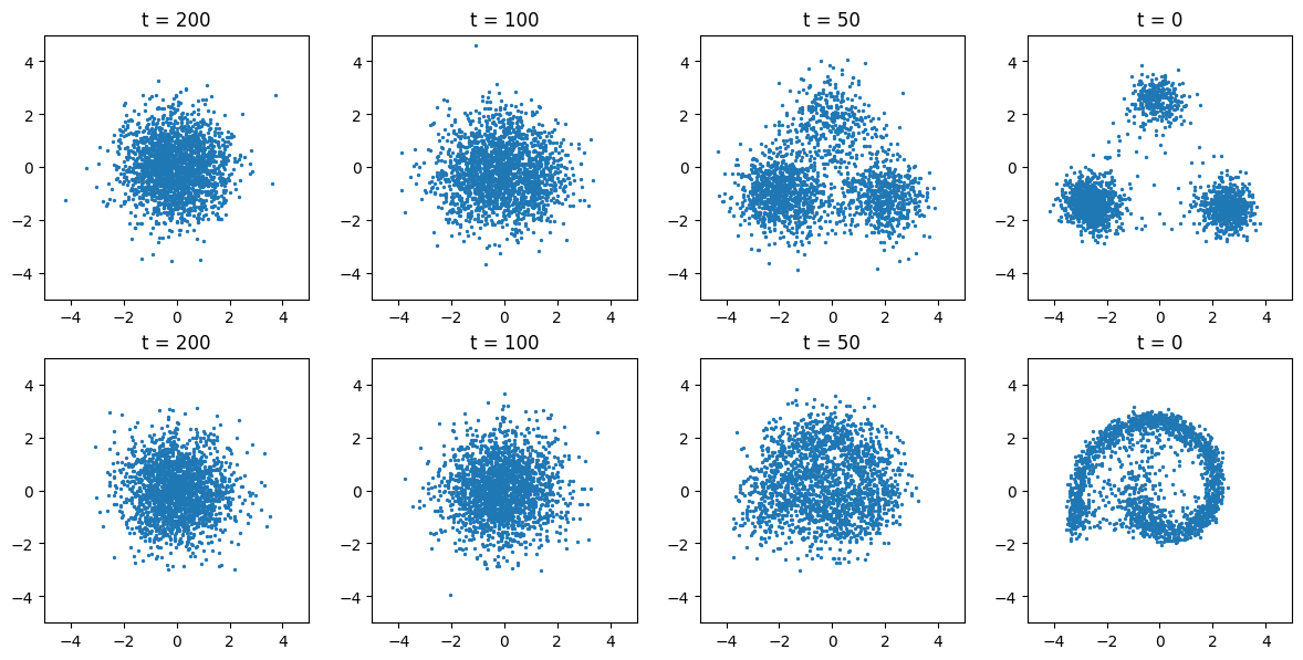
Two hundred steps from a Gaussian cloud: no structure at half the schedule, the mixture’s layout by t = 50, detail at the end. The sampler adds no parameters beyond the forward schedule and \sigma_t^2 = \beta_t.
Recap
- Forward: a fixed variance-preserving chain with closed-form marginals.
- Reverse: Gaussian transitions with learned means; the bound splits into per-step Kullback–Leibler terms, and training uses its unweighted simplification.
- Noise prediction turns every term into a regression; the simple loss is reweighted denoising score matching.
- Sampling is Langevin-like with a fixed schedule. Next: the same model on images, with a U-Net and class conditioning.