@torch.no_grad()
def ddim_sample(eps_model, x, steps, eta=0.0, record=False):
    """Sample with (eta = 0) or without (eta > 0) determinism on `steps` steps."""
    taus = torch.linspace(T - 1, 0, steps).round().long().tolist()
    a_bars = [alpha_bar[t].item() for t in taus] + [1.0]  # ends at the clean point
    trajectory = [x]
    for k, t in enumerate(taus):
        a_t, a_s = a_bars[k], a_bars[k + 1]
        eps = eps_model(x, torch.full((len(x),), t))
        x0_hat = (x - (1 - a_t) ** 0.5 * eps) / a_t ** 0.5
        sigma = eta * ((1 - a_s) / (1 - a_t) * (1 - a_t / a_s)) ** 0.5 if a_s < 1 else 0
        x = (a_s ** 0.5 * x0_hat + max(1 - a_s - sigma ** 2, 0) ** 0.5 * eps
             + sigma * torch.randn_like(x))
        trajectory.append(x)
    return (x, torch.stack(trajectory)) if record else x

torch.manual_seed(3)
x_T = torch.randn(2000, 2)
print(f'target (2000 samples of the mixture): {summarize(data)}')
print(f'DDPM, 200 steps (eta = 1): {summarize(ddim_sample(net, x_T, 200, eta=1.0))}')
for steps in (200, 50, 20, 10):
print(f'DDIM, {steps:>3d} steps (eta = 0): {summarize(ddim_sample(net, x_T, steps))}')Denoising Diffusion Implicit Models
Dive into Deep Learning · §17.9
Denoising diffusion implicit models
the same marginals, many forward processes · a deterministic sampler · skipping steps
Training Sees Only the Marginals
L_{\textrm{simple}} = \mathbb{E}_{t, \mathbf{x}_0, \boldsymbol{\epsilon}} \big\| \boldsymbol{\epsilon} - \boldsymbol{\epsilon}_{\boldsymbol{\theta}}\big(\sqrt{\bar{\alpha}_t}\, \mathbf{x}_0 + \sqrt{1 - \bar{\alpha}_t}\, \boldsymbol{\epsilon},\ t\big) \big\|^2
- only q(\mathbf{x}_t \mid \mathbf{x}_0) enters, never the chain;
- any forward process with these marginals is served by the same network, up to the weighting;
- so choose the forward process for the sampler we want.
A Non-Markovian Family with DDPM’s Marginals
q_\sigma(\mathbf{x}_{t-1} \mid \mathbf{x}_t, \mathbf{x}_0) = \mathcal{N}\!\left( \sqrt{\bar{\alpha}_{t-1}}\, \mathbf{x}_0 + \sqrt{1 - \bar{\alpha}_{t-1} - \sigma_t^2}\; \frac{\mathbf{x}_t - \sqrt{\bar{\alpha}_t}\, \mathbf{x}_0}{\sqrt{1 - \bar{\alpha}_t}},\ \sigma_t^2 I \right)
- marginals \mathcal{N}(\sqrt{\bar{\alpha}_t}\, \mathbf{x}_0, (1 - \bar{\alpha}_t) I) for every \sigma;
- \sigma_t^2 = \tilde{\beta}_t: the DDPM chain; \sigma_t = 0: deterministic given \mathbf{x}_0.
The DDIM Update
\mathbf{x}_{t-1} = \sqrt{\bar{\alpha}_{t-1}}\; \hat{\mathbf{x}}_0 + \sqrt{1 - \bar{\alpha}_{t-1} - \sigma_t^2}\; \boldsymbol{\epsilon}_{\boldsymbol{\theta}}(\mathbf{x}_t, t) + \sigma_t \mathbf{z}, \qquad \hat{\mathbf{x}}_0 = \frac{\mathbf{x}_t - \sqrt{1 - \bar{\alpha}_t}\; \boldsymbol{\epsilon}_{\boldsymbol{\theta}}}{\sqrt{\bar{\alpha}_t}}
Predict the clean point, re-noise it to the next level, add \sigma_t noise. \eta scales \sigma_t from DDIM (0) to DDPM with the posterior variance (1); steps may be skipped.
Fifty Steps Do the Work of Two Hundred
target (2000 samples of the mixture): mode weights [0.5, 0.317, 0.183], spread 0.49, stray 0.012
DDPM, 200 steps (eta = 1): mode weights [0.515, 0.32, 0.166], spread 0.44, stray 0.024
DDIM, 200 steps (eta = 0): mode weights [0.492, 0.359, 0.148], spread 0.47, stray 0.065
DDIM,  50 steps (eta = 0): mode weights [0.502, 0.359, 0.139], spread 0.46, stray 0.066
DDIM,  20 steps (eta = 0): mode weights [0.511, 0.357, 0.132], spread 0.47, stray 0.068
DDIM,  10 steps (eta = 0): mode weights [0.497, 0.375, 0.127], spread 0.41, stray 0.082
Long strides contract the spread; with the exact predictor the stride error grows from hundredths to about half a unit between fifty and five steps.
Two Samplers, Same Starting Points
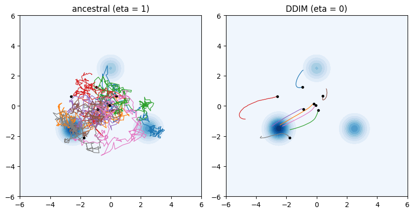
The ancestral chain wanders; the deterministic one follows a smooth curve.
Images: 1000 versus 50 versus 10 Evaluations
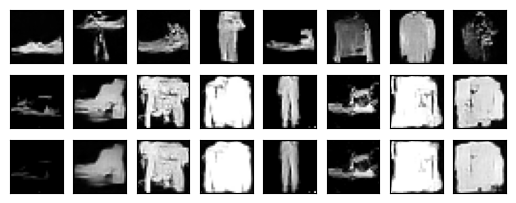
rows: ancestral, 1000 steps | DDIM, 50 steps | DDIM, 10 stepsRows two and three resemble each other column by column: the code determines the image. The stochastic row is cleaner for this small model; the gain is in cost.
Interpolating in Code Space

Codes along a great circle between two noise images decode, with fifty deterministic steps, to images that change gradually.
Recap
- DDPM’s objective fixes only the marginals; a non-Markovian family shares them, and one trained network serves all of it.
- DDIM: deterministic reverse update, \eta interpolates back to DDPM with the posterior variance, steps can be skipped at a measurable cost.
- Determinism turns \mathbf{x}_T into a code: consistency, interpolation, inversion.
- Small steps integrate an ODE. Next: velocities and flow matching.