Implementing cross-correlation

Convolutions for Images

Why convolution works for images

A fully-connected layer on a 1-megapixel RGB image needs roughly 3 million weights per output unit — wildly wasteful, since pixel correlations are local and the same edge detector should work everywhere.

A convolutional layer swaps this for two strong inductive biases:

Translation invariance — one small filter, slid everywhere with shared parameters.
Locality — each output depends only on a small neighborhood of input pixels.

Thousands of parameters instead of millions, with exactly the right prior for natural images.

2-D cross-correlation

Slide a small kernel \mathbf{K} over the input \mathbf{X}. At each position, multiply elementwise and sum:

Y[i, j] = \sum_{a, b} X[i+a, j+b]\, K[a, b].

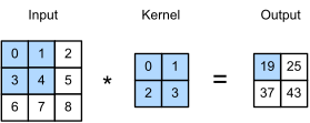
Cross-correlation: 3×3 input × 2×2 kernel → 2×2 output. Shaded element: 0{\cdot}0 + 1{\cdot}1 + 3{\cdot}2 + 4{\cdot}3 = 19.

The output is smaller than the input by k - 1 in each direction — same shrinking we’ll undo with padding next section.

Setup for implementation

Two nested loops over output positions. Each cell is a slice multiplied elementwise with the kernel and summed:

from d2l import torch as d2l
import torch
from torch import nn

def corr2d(X, K):
    """Compute 2D cross-correlation."""
    h, w = K.shape
    Y = d2l.zeros((X.shape[0] - h + 1, X.shape[1] - w + 1))
    for i in range(Y.shape[0]):
        for j in range(Y.shape[1]):
            Y[i, j] = d2l.reduce_sum((X[i: i + h, j: j + w] * K))
    return Y

Verify cross-correlation

Verify against the figure — 3×3 input × 2×2 kernel → 2×2 output with the worked-out values:

X = d2l.tensor([[0.0, 1.0, 2.0], [3.0, 4.0, 5.0], [6.0, 7.0, 8.0]])
K = d2l.tensor([[0.0, 1.0], [2.0, 3.0]])
corr2d(X, K)

tensor([[19., 25.],
        [37., 43.]])

A conv layer is corr2d + bias

Wrap the operator as a learnable Module. Two parameters: the kernel weights and a scalar bias:

class Conv2D(nn.Module):
    def __init__(self, kernel_size):
        super().__init__()
        self.weight = nn.Parameter(torch.rand(kernel_size))
        self.bias = nn.Parameter(torch.zeros(1))

    def forward(self, x):
        return corr2d(x, self.weight) + self.bias

These are the only learnable parameters of a single-channel conv layer. A 3×3 conv has nine weights regardless of input size — that’s the parameter savings the inductive bias buys us.

What kernels actually do: edge detection

Build an image with a vertical edge in the middle: 1s on the outsides, 0s in the middle four columns:

X = d2l.ones((6, 8))
X[:, 2:6] = 0
X

tensor([[1., 1., 0., 0., 0., 0., 1., 1.],
        [1., 1., 0., 0., 0., 0., 1., 1.],
        [1., 1., 0., 0., 0., 0., 1., 1.],
        [1., 1., 0., 0., 0., 0., 1., 1.],
        [1., 1., 0., 0., 0., 0., 1., 1.],
        [1., 1., 0., 0., 0., 0., 1., 1.]])

A 1×2 horizontal-difference kernel — discrete first derivative across x:

\mathbf{K} = [\,1, \, -1\,] \;\Rightarrow\; (\mathbf{K} * \mathbf{X})[i, j] = X[i, j] - X[i, j+1].

K = d2l.tensor([[1.0, -1.0]])

The output is the edge map

Cross-correlate the image with the difference kernel: +1 at each white→black transition, -1 at each black→white, zero everywhere else:

Y = corr2d(X, K)
Y

tensor([[ 0.,  1.,  0.,  0.,  0., -1.,  0.],
        [ 0.,  1.,  0.,  0.,  0., -1.,  0.],
        [ 0.,  1.,  0.,  0.,  0., -1.,  0.],
        [ 0.,  1.,  0.,  0.,  0., -1.,  0.],
        [ 0.,  1.,  0.,  0.,  0., -1.,  0.],
        [ 0.,  1.,  0.,  0.,  0., -1.,  0.]])

Transpose the image so the edge is now horizontal — the same kernel detects nothing:

corr2d(d2l.transpose(X), K)

tensor([[0., 0., 0., 0., 0.],
        [0., 0., 0., 0., 0.],
        [0., 0., 0., 0., 0.],
        [0., 0., 0., 0., 0.],
        [0., 0., 0., 0., 0.],
        [0., 0., 0., 0., 0.],
        [0., 0., 0., 0., 0.],
        [0., 0., 0., 0., 0.]])

Filters are direction-sensitive. Real ConvNets stack many filters per layer to cover all directions / patterns.

Learning the kernel

We don’t have to design kernels by hand. Random init, SGD on squared error against ground truth \mathbf{Y}:

# Construct a two-dimensional convolutional layer with 1 output channel and a
# kernel of shape (1, 2). For the sake of simplicity, we ignore the bias here
conv2d = nn.LazyConv2d(1, kernel_size=(1, 2), bias=False)

# The two-dimensional convolutional layer uses four-dimensional input and
# output in the format of (example, channel, height, width), where the batch
# size (number of examples in the batch) and the number of channels are both 1
X = X.reshape((1, 1, 6, 8))
Y = Y.reshape((1, 1, 6, 7))
lr = 3e-2  # Learning rate

for i in range(10):
    Y_hat = conv2d(X)
    l = (Y_hat - Y) ** 2
    conv2d.zero_grad()
    l.sum().backward()
    # Update the kernel
    conv2d.weight.data[:] -= lr * conv2d.weight.grad
    if (i + 1) % 2 == 0:
        print(f'epoch {i + 1}, loss {l.sum():.3f}')

epoch 2, loss 6.645
epoch 4, loss 1.649
epoch 6, loss 0.496
epoch 8, loss 0.173
epoch 10, loss 0.066

After 10 steps the loss is near zero, and the learned kernel is essentially [1, -1]:

d2l.reshape(conv2d.weight.data, (1, 2))

tensor([[ 1.0148, -0.9633]])

The rest of the chapter is built on this idea — let gradient descent discover what filters the data needs.

Receptive field: stacking deepens reach

The receptive field of an output cell = the set of input positions that can affect it.

A 2×2 kernel: receptive field = 2×2 pixels.
Two stacked 2×2 layers: each output cell sees 3×3 input.
Stack L layers of 3×3: \approx (2L + 1) \times (2L + 1).

Local kernels + depth = global reach without the parameter cost of large kernels.

Trained filters look biological

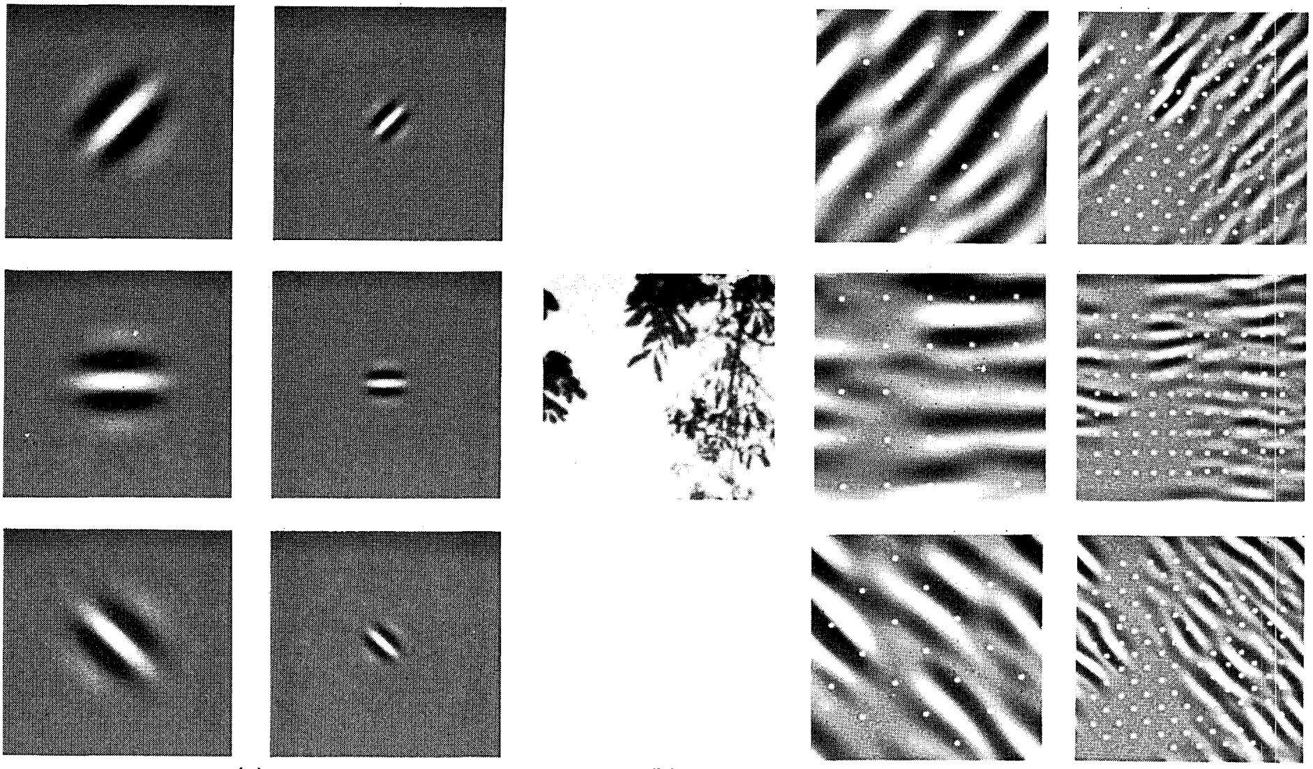
Hubel & Wiesel-style filters in the visual cortex. Trained CNN filters look strikingly similar.

Recap

Conv layer = small kernel slid across input + bias.
Inductive biases: translation invariance + locality → orders of magnitude fewer parameters than fully connected.
Hand-designed kernels can detect edges, blobs, blurs; trained kernels discover whatever the loss demands.
Receptive fields grow with depth — a deep stack of small kernels covers a large input region.
Filters look biologically plausible: the same shapes visual cortex neurons respond to.