from d2l import torch as d2l
import torch
from torch import nn
from torch.nn import functional as FResidual Networks: ResNet, ResNeXt, and DenseNet
ResNet learns residuals
ResNet (He et al., 2015) is the architecture that finally made very deep networks trainable. The key:
\mathbf{y} = f(\mathbf{x}) + \mathbf{x}.
The function only needs to learn the residual relative to identity. Identity is always representable, so adding more layers can’t hurt: 18 → 152 layers genuinely improves accuracy. Gradients flow through the skip at full strength, so deep nets train as easily as shallow ones.
Residual block
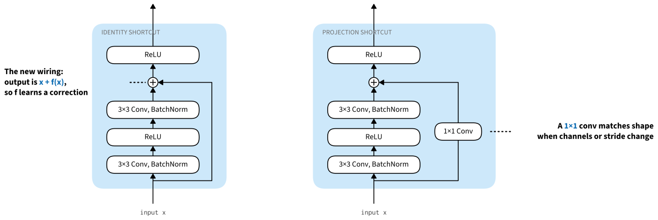
The two block variants: identity skip when shapes match, 1×1 projection on the skip path when channels or resolution change.
Block in code
A 2-conv block with a skip-add. Optional 1×1 conv on the skip path matches channel/stride changes:
class Residual(nn.Module):
    """The Residual block of ResNet models."""
    def __init__(self, num_channels, use_1x1conv=False, strides=1):
        super().__init__()
        self.conv1 = nn.LazyConv2d(num_channels, kernel_size=3, padding=1,
                                   stride=strides)
        self.conv2 = nn.LazyConv2d(num_channels, kernel_size=3, padding=1)
        # Auto-enable 1x1 conv when downsampling so the residual shape matches.
        if use_1x1conv or strides != 1:
            self.conv3 = nn.LazyConv2d(num_channels, kernel_size=1,
                                       stride=strides)
        else:
            self.conv3 = None
        self.bn1 = nn.LazyBatchNorm2d()
        self.bn2 = nn.LazyBatchNorm2d()

    def forward(self, X):
        Y = F.relu(self.bn1(self.conv1(X)))
        Y = self.bn2(self.conv2(Y))
        if self.conv3:
            X = self.conv3(X)
        Y += X
        return F.relu(Y)
Block variants
Same shape in, same shape out:
torch.Size([4, 3, 6, 6])The ResNet model
Stages of N residual blocks, with downsampling at the start of each stage:
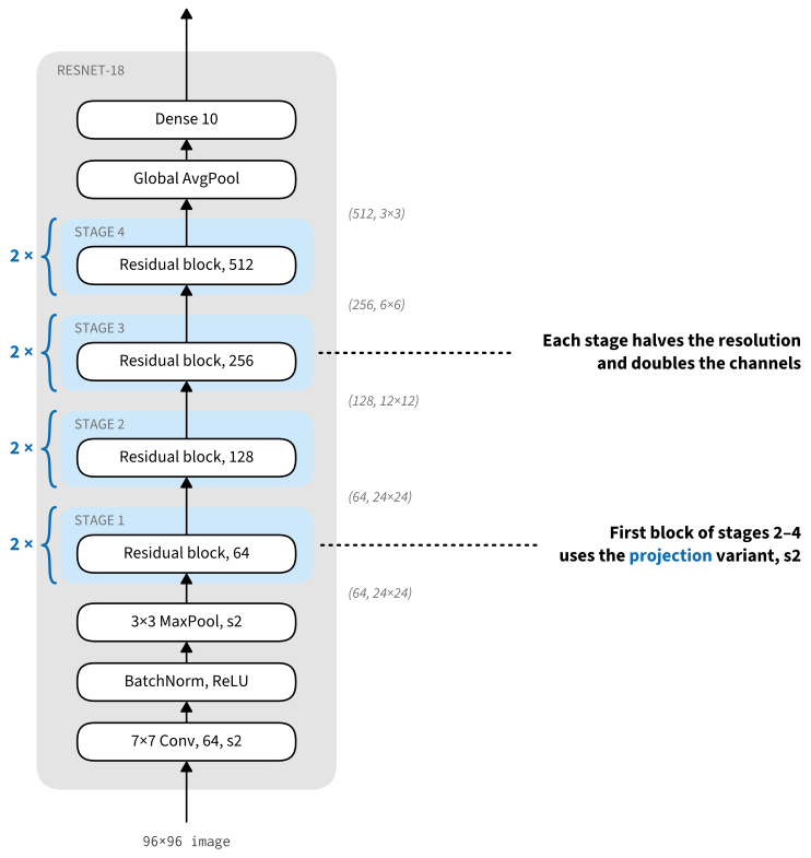
ResNet-18: four stages of two residual blocks each, plus stem and head.
ResNet stem
The stem does early feature extraction and spatial reduction, similar to AlexNet and GoogLeNet:
Residual stages
A stage is a stack of residual blocks. The first block can downsample and project the skip path; later blocks keep shape.
ResNet head
After the residual stages, global average pooling collapses the spatial map and the final linear layer predicts classes.
def __init__(self, arch, lr=0.1, num_classes=10):
    super(ResNet, self).__init__()
    self.save_hyperparameters()
    self.net = nn.Sequential(self.b1())
    for i, b in enumerate(arch):
        self.net.add_module(f'b{i+2}', self.block(*b, first_block=(i==0)))
    self.net.add_module('last', nn.Sequential(
        nn.AdaptiveAvgPool2d((1, 1)), nn.Flatten(),
        nn.LazyLinear(num_classes)))
    self.net.apply(d2l.init_cnn)
ResNet-18 assembly
Four stages × 2 residual blocks each; the same template defines ResNet-34/50/101/152:
Sequential output shape:     torch.Size([1, 64, 24, 24])
Sequential output shape:     torch.Size([1, 64, 24, 24])
Sequential output shape:     torch.Size([1, 128, 12, 12])
Sequential output shape:     torch.Size([1, 256, 6, 6])
Sequential output shape:     torch.Size([1, 512, 3, 3])
Sequential output shape:     torch.Size([1, 10])
Training
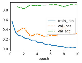
The notebook trains a compact ResNet-18 variant on Fashion-MNIST; the point is to validate that the residual-stage template plugs into the same Trainer used by earlier CNNs.
ResNeXt: width via cardinality
A cleaner variant: each block has multiple parallel paths (cardinality C) instead of one wide one, with the same parameter budget and better accuracy:
class ResNeXtBlock(nn.Module):
    """The ResNeXt block."""
    def __init__(self, num_channels, groups, bot_mul, use_1x1conv=False,
                 strides=1):
        super().__init__()
        bot_channels = int(round(num_channels * bot_mul))
        self.conv1 = nn.LazyConv2d(bot_channels, kernel_size=1, stride=1)
        self.conv2 = nn.LazyConv2d(bot_channels, kernel_size=3,
                                   stride=strides, padding=1,
                                   groups=groups)
        self.conv3 = nn.LazyConv2d(num_channels, kernel_size=1, stride=1)
        self.bn1 = nn.LazyBatchNorm2d()
        self.bn2 = nn.LazyBatchNorm2d()
        self.bn3 = nn.LazyBatchNorm2d()
        if use_1x1conv:
            self.conv4 = nn.LazyConv2d(num_channels, kernel_size=1,
                                       stride=strides)
            self.bn4 = nn.LazyBatchNorm2d()
        else:
            self.conv4 = None

    def forward(self, X):
        Y = F.relu(self.bn1(self.conv1(X)))
        Y = F.relu(self.bn2(self.conv2(Y)))
        Y = self.bn3(self.conv3(Y))
        if self.conv4:
            X = self.bn4(self.conv4(X))
        return F.relu(Y + X)
Grouped-conv savings
Grouped convolution cuts the expensive 3×3 channel mixing by a factor of groups, while surrounding 1×1 convolutions let information mix before and after the grouped work.
torch.Size([4, 32, 96, 96])DenseNet: concatenate instead of add
DenseNet (Huang et al., 2017) keeps more than two Taylor terms: instead of adding a layer’s output to its input, concatenate them along the channel dimension.
\mathbf{x}_\ell = f_\ell\bigl(\left[\mathbf{x}_0, \mathbf{x}_1, \ldots, \mathbf{x}_{\ell-1}\right]\bigr).
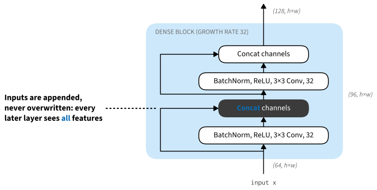
Addition keeps channels fixed; concatenation grows them, and every layer sees all earlier features.
Dense blocks in code
A conv block (BN → ReLU → 3×3 conv) is the unit; a dense block stacks them, concatenating each output onto the running input:
class DenseBlock(nn.Module):
    def __init__(self, num_convs, num_channels):
        super(DenseBlock, self).__init__()
        layer = []
        for i in range(num_convs):
            layer.append(conv_block(num_channels))
        self.net = nn.Sequential(*layer)

    def forward(self, X):
        for blk in self.net:
            Y = blk(X)
            # Concatenate input and output of each block along the channels
            X = torch.cat((X, Y), dim=1)
        return X
Transition layers, and why addition won
Each dense block grows channels by num_convs * num_channels; a transition layer (1×1 conv + 2×2 avg-pool) shrinks them back:
Feature reuse makes DenseNet parameter-efficient, but every concatenated map must stay in memory for later layers. That memory bill is why addition won at scale.
Recap
- Residual connection: \mathbf{y} = f(\mathbf{x}) + \mathbf{x}, which guarantees identity is always representable.
- Trains networks arbitrarily deep (152, 1000+) without optimization pathologies.
- ResNeXt adds cardinality: grouped 3×3 conv between 1×1 mixers.
- DenseNet concatenates instead of adds: maximal feature reuse, fewer parameters, but a memory bill that addition avoids.
- The “residual block” + “stage” template is universal: used in vision (ResNet, ResNeXt), language (Transformers, all use residual + LayerNorm), and beyond.
- ResNet-50 is the default ImageNet backbone for transfer learning even a decade later.