The NiN model

Network in Network (NiN)

NiN: MLPs inside convolutions

Network-in-Network (Lin et al., 2014) introduces two ideas the rest of the field happily adopts:

• 1×1 convolutions as a lightweight “MLP per pixel” — adds nonlinearity and channel mixing without spatial cost.
• Global average pooling replaces the giant FC classifier head — huge parameter reduction.

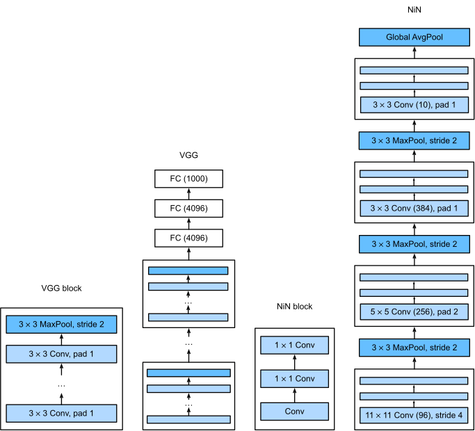
NiN: regular conv followed by two 1×1 convs; ends in global average pool.

The NiN block

A regular conv followed by two 1×1 convs (with ReLU between) — the “MLP within a conv layer”:

from d2l import torch as d2l
import torch
from torch import nn

def nin_block(out_channels, kernel_size, strides, padding):
    return nn.Sequential(
        nn.LazyConv2d(out_channels, kernel_size, strides, padding), nn.ReLU(),
        nn.LazyConv2d(out_channels, kernel_size=1), nn.ReLU(),
        nn.LazyConv2d(out_channels, kernel_size=1), nn.ReLU())

Four NiN blocks at growing channel counts (96, 256, 384, num_classes), with max-pool downsampling between, then global average pooling + flatten → done. No FC layers.

class NiN(d2l.Classifier):
    def __init__(self, lr=0.1, num_classes=10):
        super().__init__()
        self.save_hyperparameters()
        self.net = nn.Sequential(
            nin_block(96, kernel_size=11, strides=4, padding=0),
            nn.MaxPool2d(3, stride=2),
            nin_block(256, kernel_size=5, strides=1, padding=2),
            nn.MaxPool2d(3, stride=2),
            nin_block(384, kernel_size=3, strides=1, padding=1),
            nn.MaxPool2d(3, stride=2),
            nn.Dropout(0.5),
            nin_block(num_classes, kernel_size=3, strides=1, padding=1),
            nn.AdaptiveAvgPool2d((1, 1)),
            nn.Flatten())
        self.net.apply(d2l.init_cnn)

Shape inspection

Walk a 1×1×224×224 input through; spatial dims shrink, channels grow until the final block produces num_classes channels:

NiN().layer_summary((1, 1, 224, 224))

Sequential output shape:     torch.Size([1, 96, 54, 54])
MaxPool2d output shape:  torch.Size([1, 96, 26, 26])
Sequential output shape:     torch.Size([1, 256, 26, 26])
MaxPool2d output shape:  torch.Size([1, 256, 12, 12])
Sequential output shape:     torch.Size([1, 384, 12, 12])
MaxPool2d output shape:  torch.Size([1, 384, 5, 5])
Dropout output shape:    torch.Size([1, 384, 5, 5])
Sequential output shape:     torch.Size([1, 10, 5, 5])
AdaptiveAvgPool2d output shape:  torch.Size([1, 10, 1, 1])
Flatten output shape:    torch.Size([1, 10])

Training

Same Trainer, slightly higher learning rate than the FC nets (no dense layer to overfit on small batches):

model = NiN(lr=0.05)
trainer = d2l.Trainer(max_epochs=10, num_gpus=1)
data = d2l.FashionMNIST(batch_size=128, resize=(224, 224))
model.apply_init([next(iter(data.get_dataloader(True)))[0]], d2l.init_cnn)
trainer.fit(model, data)

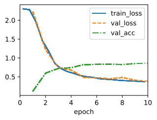
The important comparison is parameter economy: accuracy comes from richer convolutional blocks, not a large fully connected head.

Recap

• NiN puts an MLP inside each conv block via two 1×1 convs.
• Global average pooling as the classifier head — one number per class per feature map, no FC layers needed.
• The 1×1 conv as channel-mixer becomes a foundational primitive in all later architectures.
• Despite never winning a major benchmark, NiN’s ideas are in every ConvNet that came after.