GoogLeNet stem and early stages

Multi-Branch Networks (GoogLeNet)

GoogLeNet goes wide

GoogLeNet (Szegedy et al., 2014) — winner of ImageNet 2014 — introduces a different design axis: width, not just depth.

Each layer is an Inception block that runs multiple filter sizes in parallel (1×1, 3×3, 5×5, plus pool) and concatenates their outputs. The network can choose, layer by layer, which scale of filter is most useful.

Heavy use of 1×1 convs as bottleneck reductions keeps the parameter count manageable despite the multi-branch design.

Inception block

Four parallel branches at the same spatial size, concatenated along the channel axis:

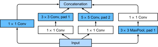
Inception: four parallel branches, channel-concatenated.

The four branches

• 1: 1×1 conv (small filter only)
• 2: 1×1 conv → 3×3 conv (with bottleneck)
• 3: 1×1 conv → 5×5 conv (with bottleneck)
• 4: 3×3 max-pool → 1×1 conv

from d2l import torch as d2l
import torch
from torch import nn
from torch.nn import functional as F

class Inception(nn.Module):
    # c1--c4 are the number of output channels for each branch
    def __init__(self, c1, c2, c3, c4, **kwargs):
        super(Inception, self).__init__(**kwargs)
        # Branch 1
        self.b1_1 = nn.LazyConv2d(c1, kernel_size=1)
        # Branch 2
        self.b2_1 = nn.LazyConv2d(c2[0], kernel_size=1)
        self.b2_2 = nn.LazyConv2d(c2[1], kernel_size=3, padding=1)
        # Branch 3
        self.b3_1 = nn.LazyConv2d(c3[0], kernel_size=1)
        self.b3_2 = nn.LazyConv2d(c3[1], kernel_size=5, padding=2)
        # Branch 4
        self.b4_1 = nn.MaxPool2d(kernel_size=3, stride=1, padding=1)
        self.b4_2 = nn.LazyConv2d(c4, kernel_size=1)

    def forward(self, x):
        b1 = F.relu(self.b1_1(x))
        b2 = F.relu(self.b2_2(F.relu(self.b2_1(x))))
        b3 = F.relu(self.b3_2(F.relu(self.b3_1(x))))
        b4 = F.relu(self.b4_2(self.b4_1(x)))
        return torch.cat((b1, b2, b3, b4), dim=1)

Five sequential “stages” — each a small stack of conv + pool + inception modules — built up methodically. The stem and second stage reduce resolution quickly before the Inception blocks take over:

class GoogleNet(d2l.Classifier):
    def b1(self):
        return nn.Sequential(
            nn.LazyConv2d(64, kernel_size=7, stride=2, padding=3),
            nn.ReLU(), nn.MaxPool2d(kernel_size=3, stride=2, padding=1))

def b2(self):
    return nn.Sequential(
        nn.LazyConv2d(64, kernel_size=1), nn.ReLU(),
        nn.LazyConv2d(192, kernel_size=3, padding=1), nn.ReLU(),
        nn.MaxPool2d(kernel_size=3, stride=2, padding=1))

First Inception stack

Stage 3 introduces the repeating pattern: two Inception blocks, then pooling. Channel counts are split across branches, then concatenated back together.

def b3(self):
    return nn.Sequential(Inception(64, (96, 128), (16, 32), 32),
                         Inception(128, (128, 192), (32, 96), 64),
                         nn.MaxPool2d(kernel_size=3, stride=2, padding=1))

Deep Inception stages

Stage 4 is the compute-heavy middle of the network: five Inception blocks before the next spatial downsample.

def b4(self):
    return nn.Sequential(Inception(192, (96, 208), (16, 48), 64),
                         Inception(160, (112, 224), (24, 64), 64),
                         Inception(128, (128, 256), (24, 64), 64),
                         Inception(112, (144, 288), (32, 64), 64),
                         Inception(256, (160, 320), (32, 128), 128),
                         nn.MaxPool2d(kernel_size=3, stride=2, padding=1))

Head and assembly

Stage 5 uses global average pooling before the final classifier, then __init__ simply wires b1 through b5 together.

def b5(self):
    return nn.Sequential(Inception(256, (160, 320), (32, 128), 128),
                         Inception(384, (192, 384), (48, 128), 128),
                         nn.AdaptiveAvgPool2d((1,1)), nn.Flatten())

def __init__(self, lr=0.1, num_classes=10):
    super(GoogleNet, self).__init__()
    self.save_hyperparameters()
    self.net = nn.Sequential(self.b1(), self.b2(), self.b3(), self.b4(),
                             self.b5(), nn.LazyLinear(num_classes))
    self.net.apply(d2l.init_cnn)

Shape inspection

For Fashion-MNIST we shrink the input to 96×96 to keep training time reasonable; layer summary on the smaller input:

model = GoogleNet().layer_summary((1, 1, 96, 96))

Sequential output shape:     torch.Size([1, 64, 24, 24])
Sequential output shape:     torch.Size([1, 192, 12, 12])
Sequential output shape:     torch.Size([1, 480, 6, 6])
Sequential output shape:     torch.Size([1, 832, 3, 3])
Sequential output shape:     torch.Size([1, 1024])
Linear output shape:     torch.Size([1, 10])

Notice the pattern: spatial resolution falls at pools, while channel depth grows after concatenating each Inception block’s branches.

Training

model = GoogleNet(lr=0.01)
trainer = d2l.Trainer(max_epochs=10, num_gpus=1)
data = d2l.FashionMNIST(batch_size=128, resize=(96, 96))
model.apply_init([next(iter(data.get_dataloader(True)))[0]], d2l.init_cnn)
trainer.fit(model, data)

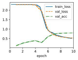
The original GoogLeNet has 22 weighted layers (~7M params) — far fewer than VGG (~138M) — yet better ImageNet accuracy.

Recap

• Inception block = multi-branch, multi-scale, concatenated. The network learns which filter size matters per layer.
• 1×1 bottlenecks keep parameter count low.
• The “go wider, not just deeper” lesson informs every modern attention/feature-pyramid design.
• GoogLeNet’s descendants (Inception-v3/v4, Xception) refined the block; the underlying multi-branch + bottleneck template endures.