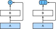
Dense block

Densely Connected Networks (DenseNet)

DenseNet concatenates features

DenseNet (Huang et al., 2017) takes the residual idea one step further: instead of adding skip connections, concatenate them.

\mathbf{x}_\ell = f_\ell\bigl([\mathbf{x}_0, \mathbf{x}_1, \dots, \mathbf{x}_{\ell-1}]\bigr).

Every layer in a dense block sees the concatenation of all preceding outputs.

Dense block + transition

Dense block grows channels by concatenation; transition layers (1×1 conv + pool) reset channels between blocks.

Pros: maximum feature reuse, fewer parameters than ResNet for similar accuracy. Cons: memory grows linearly with depth within a block — handled by transitions.

Conv block

A small conv block (BN → ReLU → 3×3 conv) is the unit; a DenseBlock will reuse it repeatedly.

from d2l import torch as d2l
import torch
from torch import nn

def conv_block(num_channels):
    return nn.Sequential(
        nn.LazyBatchNorm2d(), nn.ReLU(),
        nn.LazyConv2d(num_channels, kernel_size=3, padding=1))

Now stack the conv blocks. After each block, concatenate its new features onto the running input, so later blocks see everything computed so far.

class DenseBlock(nn.Module):
    def __init__(self, num_convs, num_channels):
        super(DenseBlock, self).__init__()
        layer = []
        for i in range(num_convs):
            layer.append(conv_block(num_channels))
        self.net = nn.Sequential(*layer)

    def forward(self, X):
        for blk in self.net:
            Y = blk(X)
            # Concatenate input and output of each block along the channels
            X = torch.cat((X, Y), dim=1)
        return X

Channel growth

A DenseBlock(num_convs=2, num_channels=10) on a 3-channel input grows channels by num_convs * num_channels per block:

blk = DenseBlock(2, 10)
X = torch.randn(4, 3, 8, 8)
Y = blk(X)
Y.shape

torch.Size([4, 23, 8, 8])

Transition layer

Stops the channel explosion between dense blocks: 1×1 conv halves channels, 2×2 avg-pool halves spatial dims:

def transition_block(num_channels):
    return nn.Sequential(
        nn.LazyBatchNorm2d(), nn.ReLU(),
        nn.LazyConv2d(num_channels, kernel_size=1),
        nn.AvgPool2d(kernel_size=2, stride=2))

blk = transition_block(10)
blk(Y).shape

torch.Size([4, 10, 4, 4])

The DenseNet model

A standard “stem → dense block → transition → dense block → transition → … → global avg-pool → linear” pipeline:

class DenseNet(d2l.Classifier):
    def b1(self):
        return nn.Sequential(
            nn.LazyConv2d(64, kernel_size=7, stride=2, padding=3),
            nn.LazyBatchNorm2d(), nn.ReLU(),
            nn.MaxPool2d(kernel_size=3, stride=2, padding=1))

def __init__(self, num_channels=64, growth_rate=32, arch=(4, 4, 4, 4),
             lr=0.1, num_classes=10):
    super(DenseNet, self).__init__()
    self.save_hyperparameters()
    self.net = nn.Sequential(self.b1())
    for i, num_convs in enumerate(arch):
        self.net.add_module(f'dense_blk{i+1}', DenseBlock(num_convs,
                                                          growth_rate))
        # The number of output channels in the previous dense block
        num_channels += num_convs * growth_rate
        # A transition layer that halves the number of channels is added
        # between the dense blocks
        if i != len(arch) - 1:
            num_channels //= 2
            self.net.add_module(f'tran_blk{i+1}', transition_block(
                num_channels))
    self.net.add_module('last', nn.Sequential(
        nn.LazyBatchNorm2d(), nn.ReLU(),
        nn.AdaptiveAvgPool2d((1, 1)), nn.Flatten(),
        nn.LazyLinear(num_classes)))
    self.net.apply(d2l.init_cnn)

Training

model = DenseNet(lr=0.01)
trainer = d2l.Trainer(max_epochs=10, num_gpus=1)
data = d2l.FashionMNIST(batch_size=128, resize=(96, 96))
trainer.fit(model, data)

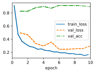
DenseNet hits competitive ImageNet accuracy with far fewer parameters than equivalent ResNets — the concatenation reuse genuinely helps.

Recap

• ResNet adds skip connections; DenseNet concatenates them.
• Inside a dense block, layer \ell sees all of layers 0, …, \ell-1 — maximum feature reuse.
• Transition layers between dense blocks rein in the channel-count explosion via 1×1 conv + pool.
• Same parameter count → typically better accuracy than ResNet; same accuracy → fewer parameters.