Normalization Layers

BatchNorm stabilizes deep nets

Batch Normalization (Ioffe & Szegedy, 2015) is the single-biggest stability win in modern deep learning.

At each layer, normalize activations within the minibatch to zero mean / unit variance, then rescale with learned \gamma and \beta:

\text{BN}(\mathbf{x}) = \gamma \cdot \frac{\mathbf{x} - \hat\mu_\mathcal{B}}{\sqrt{\hat\sigma_\mathcal{B}^2 + \epsilon}} + \beta.

Why it works

• Lets you train much deeper nets — gradients stay well-conditioned through the depth.
• Allows higher learning rates; mildly regularizing.
• Test time uses running estimates of mean / variance (no minibatch then).
• Spawned a family — LayerNorm (per-example, used in Transformers), GroupNorm, InstanceNorm.

From scratch

Compute per-channel mean and variance over the minibatch (and spatial dims, for conv); normalize, then scale + shift:

from d2l import torch as d2l
import torch
from torch import nn

def batch_norm(X, gamma, beta, moving_mean, moving_var, eps, momentum,
               training):
    if not training:
        # In prediction mode, use mean and variance obtained by moving average
        X_hat = (X - moving_mean) / torch.sqrt(moving_var + eps)
    else:
        assert len(X.shape) in (2, 4)
        if len(X.shape) == 2:
            # When using a fully connected layer, calculate the mean and
            # variance on the feature dimension
            mean = X.mean(dim=0)
            var = ((X - mean) ** 2).mean(dim=0)
            running_var = X.var(dim=0, unbiased=True)
        else:
            # When using a two-dimensional convolutional layer, calculate the
            # mean and variance on the channel dimension (axis=1). Here we
            # need to maintain the shape of X, so that the broadcasting
            # operation can be carried out later
            mean = X.mean(dim=(0, 2, 3), keepdim=True)
            var = ((X - mean) ** 2).mean(dim=(0, 2, 3), keepdim=True)
            running_var = X.var(dim=(0, 2, 3), unbiased=True, keepdim=True)
        # In training mode, the current mean and variance are used 
        X_hat = (X - mean) / torch.sqrt(var + eps)
        # Update the mean and variance using moving average
        moving_mean = (1.0 - momentum) * moving_mean + momentum * mean
        moving_var = ((1.0 - momentum) * moving_var
                      + momentum * running_var)
    Y = gamma * X_hat + beta  # Scale and shift
    return Y, moving_mean.detach(), moving_var.detach()

Wrapping as a Module

Buffers for moving_mean / moving_var (updated only during training); learnable gamma / beta parameters:

class BatchNorm(nn.Module):
    # num_features: the number of outputs for a fully connected layer or the
    # number of output channels for a convolutional layer. num_dims: 2 for a
    # fully connected layer and 4 for a convolutional layer
    def __init__(self, num_features, num_dims):
        super().__init__()
        if num_dims == 2:
            shape = (1, num_features)
        else:
            shape = (1, num_features, 1, 1)
        # The scale parameter and the shift parameter (model parameters) are
        # initialized to 1 and 0, respectively
        self.gamma = nn.Parameter(torch.ones(shape))
        self.beta = nn.Parameter(torch.zeros(shape))
        # The variables that are not model parameters are initialized to 0 and
        # 1
        self.register_buffer('moving_mean', torch.zeros(shape))
        self.register_buffer('moving_var', torch.ones(shape))

    def forward(self, X):
        Y, moving_mean, moving_var = batch_norm(
            X, self.gamma, self.beta, self.moving_mean,
            self.moving_var, eps=1e-5, momentum=0.1,
            training=self.training)
        self.moving_mean.copy_(moving_mean)
        self.moving_var.copy_(moving_var)
        return Y

LeNet + BatchNorm

Drop a BatchNorm layer between each conv/linear and its activation:

class BNLeNetScratch(d2l.Classifier):
    def __init__(self, lr=0.1, num_classes=10):
        super().__init__()
        self.save_hyperparameters()
        self.net = nn.Sequential(
            nn.LazyConv2d(6, kernel_size=5), BatchNorm(6, num_dims=4),
            nn.Sigmoid(), nn.AvgPool2d(kernel_size=2, stride=2),
            nn.LazyConv2d(16, kernel_size=5), BatchNorm(16, num_dims=4),
            nn.Sigmoid(), nn.AvgPool2d(kernel_size=2, stride=2),
            nn.Flatten(), nn.LazyLinear(120),
            BatchNorm(120, num_dims=2), nn.Sigmoid(), nn.LazyLinear(84),
            BatchNorm(84, num_dims=2), nn.Sigmoid(),
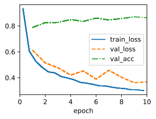
            nn.LazyLinear(num_classes))

Train

Trains noticeably faster than vanilla LeNet — same accuracy in fewer epochs:

trainer = d2l.Trainer(max_epochs=10, num_gpus=1)
data = d2l.FashionMNIST(batch_size=128)
model = BNLeNetScratch(lr=0.1)
model.apply_init([next(iter(data.get_dataloader(True)))[0]], d2l.init_cnn)
trainer.fit(model, data)

After training, gamma and beta are non-trivial — the layer learned the scale/shift it wants:

model.net[1].gamma.reshape((-1,)), model.net[1].beta.reshape((-1,))

(tensor([1.4442, 2.0445, 1.7394, 1.9345, 2.1598, 1.9288], device='cuda:0',
        grad_fn=<ViewBackward0>),
 tensor([-1.0764,  0.8309,  1.6231,  0.8588,  0.9734,  1.3145], device='cuda:0',
        grad_fn=<ViewBackward0>))

The framework version

nn.BatchNorm2d for conv layers, nn.BatchNorm1d for linear layers — same idea, much faster, handles the eval/training mode switch automatically:

class BNLeNet(d2l.Classifier):
    def __init__(self, lr=0.1, num_classes=10):
        super().__init__()
        self.save_hyperparameters()
        self.net = nn.Sequential(
            nn.LazyConv2d(6, kernel_size=5), nn.LazyBatchNorm2d(),
            nn.Sigmoid(), nn.AvgPool2d(kernel_size=2, stride=2),
            nn.LazyConv2d(16, kernel_size=5), nn.LazyBatchNorm2d(),
            nn.Sigmoid(), nn.AvgPool2d(kernel_size=2, stride=2),
            nn.Flatten(), nn.LazyLinear(120), nn.LazyBatchNorm1d(),
            nn.Sigmoid(), nn.LazyLinear(84), nn.LazyBatchNorm1d(),
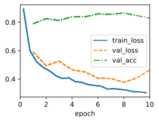
            nn.Sigmoid(), nn.LazyLinear(num_classes))

trainer = d2l.Trainer(max_epochs=10, num_gpus=1)
data = d2l.FashionMNIST(batch_size=128)
model = BNLeNet(lr=0.1)
model.apply_init([next(iter(data.get_dataloader(True)))[0]], d2l.init_cnn)
trainer.fit(model, data)

The two real problems

BatchNorm couples examples through the batch statistics:

• Minibatch coupling: the estimates degrade as batches shrink. Detection / segmentation train at 1–2 images per device.
• Train/serve discrepancy: minibatch statistics in training, moving averages at prediction. One layer, two functions.

GroupNorm (Wu & He, 2018): standardize each example within groups of channels. No batch in the statistics: batch size 1 works, and training equals serving.

GroupNorm in code

Per-(example, group) mean 0 / variance 1, at any batch size:

X = torch.randn(32, 16, 8, 8)
gn = nn.GroupNorm(4, 16)  # 4 groups of 4 channels each
Y = gn(X)
G = Y.reshape(32, 4, -1)  # Collect each (example, group) pair's elements
(G.mean(dim=2).abs().max(), G.var(dim=2, unbiased=False).mean(),
 torch.allclose(gn(X[:1]), Y[:1], atol=1e-6))

(tensor(2.4214e-08, grad_fn=<MaxBackward1>),
 tensor(1.0000, grad_fn=<MeanBackward0>),
 True)

The default in detection / segmentation heads and diffusion U-Nets, where per-device batches are small.

Recap

• BatchNorm normalizes activations to zero mean / unit variance within each minibatch, then rescales with learned \gamma, \beta.
• Track running statistics during training; use them at inference (no minibatch at test time).
• Enables much deeper networks, higher LRs, faster convergence; mildly regularizing.
• Spawned a family — LayerNorm (per-example, used in Transformers), GroupNorm, InstanceNorm.