apply(img, torchvision.transforms.RandomHorizontalFlip())Reference image
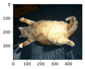
All augmentation examples start from this single image. The label is assumed to stay valid after each transform; that label-preserving assumption is what makes augmentation useful.
Flips and crops
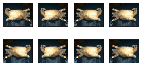
Random horizontal flip — the cheapest, most-used augmentation. It is safe when left/right orientation is not part of the label:
Vertical flip — used selectively. It is valid for some textures or aerial imagery, but usually wrong for faces, street scenes, and text:
apply(img, torchvision.transforms.RandomVerticalFlip())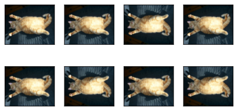
Random resized crop
Crop a random rectangle, resize back to the input size. The single most effective augmentation in vision: scale invariance and translation invariance in one trick:
shape_aug = torchvision.transforms.RandomResizedCrop(
    (200, 200), scale=(0.1, 1), ratio=(0.5, 2))
apply(img, shape_aug)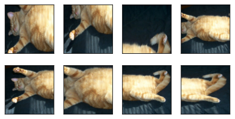
Color jitter — brightness
Brightness jitter changes illumination without moving object geometry. The object should still be recognizable across the sample grid:
apply(img, torchvision.transforms.ColorJitter(
    brightness=0.5, contrast=0, saturation=0, hue=0))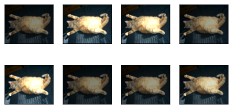
Color jitter — hue
Hue jitter changes color statistics. Use it only when color is not itself the label signal:
apply(img, torchvision.transforms.ColorJitter(
    brightness=0, contrast=0, saturation=0, hue=0.5))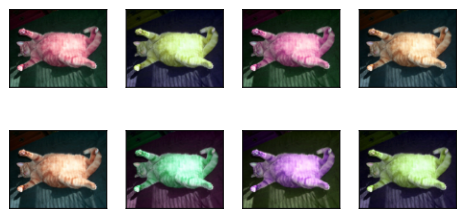
Combined color jitter
Brightness, contrast, saturation, hue — all at once. Tame the magnitudes; large jitters destroy semantic content:
color_aug = torchvision.transforms.ColorJitter(
    brightness=0.5, contrast=0.5, saturation=0.5, hue=0.5)
apply(img, color_aug)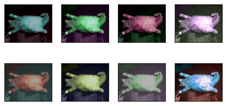
Composing augmentations
Compose([flip, crop, color, ToTensor]) — a pipeline of transforms applied in order. Standard recipe:
augs = torchvision.transforms.Compose([
    torchvision.transforms.RandomHorizontalFlip(), color_aug, shape_aug])
apply(img, augs)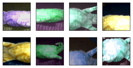
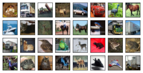
CIFAR-10 samples
The batch should still look like valid CIFAR-10 examples, just shifted, cropped, and flipped. If many objects are cropped out, the augmentation is too aggressive.
Train it
Augmentation often slows training loss at first because the problem is harder. The payoff is lower validation error from reduced overfitting.
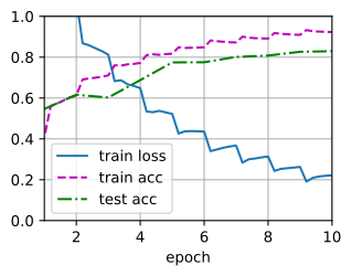
loss 0.218, train acc 0.925, test acc 0.825
7055.8 examples/sec on [device(type='cuda', index=0)]