Four kernels

Attention Pooling by Similarity

A 1964 statistics paper hides a baby attention mechanism. The Nadaraya–Watson estimator computes

\hat f(\mathbf{q}) = \sum_i \frac{\alpha(\mathbf{q}, \mathbf{k}_i)}{\sum_j \alpha(\mathbf{q}, \mathbf{k}_j)}\, \mathbf{v}_i,

with a similarity kernel \alpha playing the role of attention weights, the training inputs \mathbf{x}_i as keys, and labels y_i as values. No training, just a closed-form regressor — and it’s exactly attention pooling with hand-picked \alpha.

This deck uses N–W to visualize what attention does, and to motivate why we’d want to learn \alpha instead of fixing it.

from d2l import torch as d2l
import torch
from torch import nn
from torch.nn import functional as F
import numpy as np

d2l.use_svg_display()

Gaussian, boxcar, constant, triangular — all heuristic choices for \alpha:

# Define some kernels
def gaussian(x):
    return d2l.exp(-x**2 / 2)

def boxcar(x):
    return d2l.abs(x) < 1.0

def constant(x):
    return 1.0 + 0 * x
 
def triangular(x):
    return torch.max(1 - d2l.abs(x), torch.zeros_like(x))

Plot them on [-2.5, 2.5]:

fig, axes = d2l.plt.subplots(1, 4, sharey=True, figsize=(12, 3))

kernels = (gaussian, boxcar, constant, triangular)
names = ('Gaussian', 'Boxcar', 'Constant', 'Triangular')
x = d2l.arange(-2.5, 2.5, 0.1)
for kernel, name, ax in zip(kernels, names, axes):
    ax.plot(d2l.numpy(x), d2l.numpy(kernel(x)))
    ax.set_xlabel(name)

d2l.plt.show()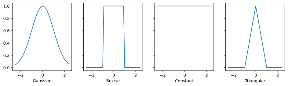

Synthetic data

y = 2\sin(x) + x + \epsilon on [0, 5], 40 noisy training points, dense validation grid:

def f(x):
    return 2 * d2l.sin(x) + x

n = 40
x_train, _ = torch.sort(d2l.rand(n) * 5)
y_train = f(x_train) + d2l.randn(n)
x_val = d2l.arange(0, 5, 0.1)
y_val = f(x_val)

Nadaraya–Watson in 6 lines

Pairwise distances → kernel → normalize columns → multiply by labels. The normalized kernel matrix is the attention weight matrix:

def nadaraya_watson(x_train, y_train, x_val, kernel):
    dists = d2l.reshape(x_train, (-1, 1)) - d2l.reshape(x_val, (1, -1))
    # Each column/row corresponds to each query/key
    k = d2l.astype(kernel(dists), d2l.float32)
    # Normalization over keys for each query
    attention_w = k / d2l.reduce_sum(k, 0)
    y_hat = y_train@attention_w
    return y_hat, attention_w

Plotting helper

Side-by-side panel for the four kernels — either fitted curve or attention heatmap, depending on the flag:

def plot(x_train, y_train, x_val, y_val, kernels, names, attention=False):
    fig, axes = d2l.plt.subplots(1, 4, sharey=True, figsize=(12, 3))
    for kernel, name, ax in zip(kernels, names, axes):
        y_hat, attention_w = nadaraya_watson(x_train, y_train, x_val, kernel)
        if attention:
            pcm = ax.imshow(d2l.numpy(attention_w), cmap='Reds')
        else:
            ax.plot(x_val, y_hat)
            ax.plot(x_val, y_val, 'm--')
            ax.plot(x_train, y_train, 'o', alpha=0.5);
        ax.set_xlabel(name)
        if not attention:
            ax.legend(['y_hat', 'y'])
    if attention:
        fig.colorbar(pcm, ax=axes, shrink=0.7)

Estimates by kernel

Gaussian, boxcar, triangular — all track the truth. Constant collapses to the dataset mean.

plot(x_train, y_train, x_val, y_val, kernels, names)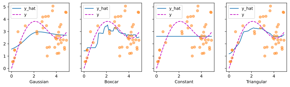

Attention weights by kernel

Heatmap view explains the agreement: the three working kernels produce near-identical attention patterns despite very different shapes:

plot(x_train, y_train, x_val, y_val, kernels, names, attention=True)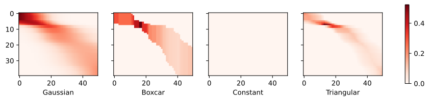

Bandwidth matters

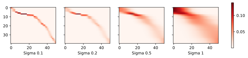
Same Gaussian, four widths. Narrower → less smooth, more local — the bias/variance trade-off shows up directly in the attention sharpness:

sigmas = (0.1, 0.2, 0.5, 1)
names = ['Sigma ' + str(sigma) for sigma in sigmas]

def gaussian_with_width(sigma): 
    return (lambda x: d2l.exp(-x**2 / (2*sigma**2)))

kernels = [gaussian_with_width(sigma) for sigma in sigmas]
plot(x_train, y_train, x_val, y_val, kernels, names)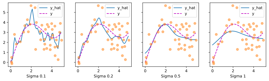

Heatmaps for varying width

As the Gaussian bandwidth grows, attention spreads across more training points. Narrow bands memorize local neighborhoods; wide bands approach a smoother global average.

plot(x_train, y_train, x_val, y_val, kernels, names, attention=True)

Recap

Nadaraya–Watson regression = attention pooling with a hand-picked similarity kernel.
Functional form of the kernel barely matters; bandwidth matters a lot.
The kernel is not learned; it’s chosen by the modeler. That’s the limitation that motivates learned attention with trainable queries and keys — coming up next.