Single Variable Calculus

Single-Variable Calculus

The single-variable calculus toolkit underlying gradient descent. The derivative

f'(x) = \lim_{\epsilon \to 0} \frac{f(x+\epsilon) - f(x)}{\epsilon}

is the local linear approximation of f at x. The gradient-descent update x \leftarrow x - \eta f'(x) uses exactly this approximation: take a small step opposite the slope.

This deck visualizes derivatives, linear approximation, and Taylor expansion — the local quadratic and beyond.

Derivative as slope of zoom

Plot a function on a normal scale, then zoom in. Smooth functions look more and more like a straight line — that line is the tangent, its slope is f'(x):

%matplotlib inline
from d2l import torch as d2l
from IPython import display
import torch
torch.pi = torch.acos(torch.zeros(1)).item() * 2  # Define pi in torch

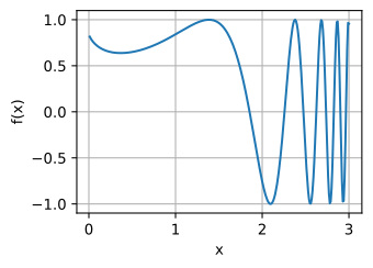
# Plot a function in a normal range
x_big = torch.arange(0.01, 3.01, 0.01)
ys = torch.sin(x_big**x_big)
d2l.plot(x_big, ys, 'x', 'f(x)')

# Plot a the same function in a tiny range
x_med = torch.arange(1.75, 2.25, 0.001)
ys = torch.sin(x_med**x_med)
d2l.plot(x_med, ys, 'x', 'f(x)')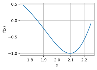

Zooming further

As the view narrows around a smooth point, curvature becomes less visible and the tangent line becomes the right local model.

# Plot a the same function in a tiny range
x_small = torch.arange(2.0, 2.01, 0.0001)
ys = torch.sin(x_small**x_small)
d2l.plot(x_small, ys, 'x', 'f(x)')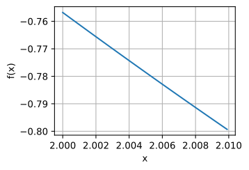

# Define our function
def L(x):
    return x**2 + 1701*(x-4)**3

# Print the difference divided by epsilon for several epsilon
for epsilon in [0.1, 0.001, 0.0001, 0.00001]:
    print(f'epsilon = {epsilon:.5f} -> {(L(4+epsilon) - L(4)) / epsilon:.5f}')

epsilon = 0.10000 -> 25.11000
epsilon = 0.00100 -> 8.00270
epsilon = 0.00010 -> 8.00012
epsilon = 0.00001 -> 8.00001

Linear approximation

f(x + \epsilon) \approx f(x) + \epsilon f'(x) — the first-order Taylor term. Valid for small \epsilon; foundation of GD analysis:

# Compute sin
xs = torch.arange(-torch.pi, torch.pi, 0.01)
plots = [torch.sin(xs)]

# Compute some linear approximations. Use d(sin(x))/dx = cos(x)
for x0 in [-1.5, 0.0, 2.0]:
    plots.append(torch.sin(torch.tensor(x0)) + (xs - x0) *
                 torch.cos(torch.tensor(x0)))

d2l.plot(xs, plots, 'x', 'f(x)', ylim=[-1.5, 1.5])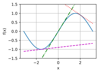

Higher-order derivatives

The second derivative measures how the slope itself changes: f''(x) > 0 curves upward, f''(x) < 0 curves downward.

# Compute sin
xs = torch.arange(-torch.pi, torch.pi, 0.01)
plots = [torch.sin(xs)]

# Compute some quadratic approximations. Use d(sin(x)) / dx = cos(x)
for x0 in [-1.5, 0.0, 2.0]:
    plots.append(torch.sin(torch.tensor(x0)) + (xs - x0) *
                 torch.cos(torch.tensor(x0)) - (xs - x0)**2 *
                 torch.sin(torch.tensor(x0)) / 2)

d2l.plot(xs, plots, 'x', 'f(x)', ylim=[-1.5, 1.5])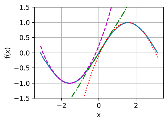

Taylor series

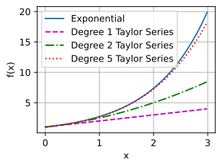
f(x + \epsilon) = \sum_{k=0}^\infty \frac{f^{(k)}(x)}{k!} \epsilon^k. Truncating gives polynomial approximations of any order:

# Compute the exponential function
xs = torch.arange(0, 3, 0.01)
ys = torch.exp(xs)

# Compute a few Taylor series approximations
P1 = 1 + xs
P2 = 1 + xs + xs**2 / 2
P5 = 1 + xs + xs**2 / 2 + xs**3 / 6 + xs**4 / 24 + xs**5 / 120

d2l.plot(xs, [ys, P1, P2, P5], 'x', 'f(x)', legend=[
    "Exponential", "Degree 1 Taylor Series", "Degree 2 Taylor Series",
    "Degree 5 Taylor Series"])

Recap

• Derivative = slope of the tangent line; second derivative = curvature.
• Linear (1st-order) Taylor → gradient descent.
• Quadratic (2nd-order) Taylor → Newton’s method.
• All of training boils down to repeatedly applying these approximations on a noisy loss landscape.