Looking at the data

Naive Bayes

Naive Bayes Classification

Naive Bayes — the simplest probabilistic classifier. Apply Bayes’ rule:

P(y \mid \mathbf{x}) \propto P(y) \prod_i P(x_i \mid y).

The “naive” part is the assumption that features are conditionally independent given the class. Wrong in general — pixels of an image are obviously correlated — but the model is fast, requires little data, and is a useful starting point.

This deck applies it to MNIST digit classification with binarized pixels.

Setup + binary MNIST

Binarize pixels so each pixel can be modeled as a Bernoulli random variable conditioned on the digit class.

%matplotlib inline
from d2l import torch as d2l
import math
import torch
import torchvision
d2l.use_svg_display()

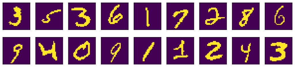
Inspect the binarized digits before fitting: the class templates are recognizable, but neighboring pixels are clearly dependent.

data_transform = torchvision.transforms.Compose([
    torchvision.transforms.ToTensor(),
    lambda x: torch.floor(x * 255 / 128).squeeze(dim=0)
])

mnist_train = torchvision.datasets.MNIST(
    root='./temp', train=True, transform=data_transform, download=True)
mnist_test = torchvision.datasets.MNIST(
    root='./temp', train=False, transform=data_transform, download=True)

0.3%
0.7%
1.0%
1.3%
1.7%
2.0%
...
93.4%
95.4%
97.4%
99.4%
100.0%
100.0%

image, label = mnist_train[2]
image.shape, label

(torch.Size([28, 28]), 4)

image.shape, image.dtype

(torch.Size([28, 28]), torch.float32)

Per-class pixel statistics

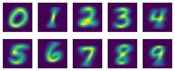
For each class y and pixel i, estimate P(x_i = 1 \mid y) from the training set. With Laplace smoothing to avoid zeros:

label, type(label)

(4, int)

images = torch.stack([mnist_train[i][0] for i in range(10, 38)], dim=0)
labels = torch.tensor([mnist_train[i][1] for i in range(10, 38)])
images.shape, labels.shape

(torch.Size([28, 28, 28]), torch.Size([28]))

d2l.show_images(images, 2, 9);

Training: just count

Training is counting, not gradient descent: estimate class priors and per-pixel likelihoods directly from the labeled examples.

X = torch.stack([mnist_train[i][0] for i in range(len(mnist_train))], dim=0)
Y = torch.tensor([mnist_train[i][1] for i in range(len(mnist_train))])

n_y = torch.zeros(10)
for y in range(10):
    n_y[y] = (Y == y).sum()
P_y = n_y / n_y.sum()
P_y

tensor([0.0987, 0.1124, 0.0993, 0.1022, 0.0974, 0.0904, 0.0986, 0.1044, 0.0975,
        0.0992])

n_x = torch.zeros((10, 28, 28))
for y in range(10):
    n_x[y] = torch.tensor(X.numpy()[Y.numpy() == y].sum(axis=0))
P_xy = (n_x + 1) / (n_y + 2).reshape(10, 1, 1)

d2l.show_images(P_xy, 2, 5);

Training (cont.)

Training stores only class priors and per-class pixel probabilities; prediction multiplies those likelihood terms, usually in log-space.

def bayes_pred(x):
    x = x.unsqueeze(0)  # (28, 28) -> (1, 28, 28)
    p_xy = P_xy * x + (1 - P_xy)*(1 - x)
    p_xy = p_xy.reshape(10, -1).prod(dim=1)  # p(x|y)
    return p_xy * P_y

image, label = mnist_test[0]
bayes_pred(image)

tensor([0., 0., 0., 0., 0., 0., 0., 0., 0., 0.])

a = 0.1
print('underflow:', a**784)
print('logarithm is normal:', 784*math.log(a))

underflow: 0.0
logarithm is normal: -1805.2267129073316

Predicting in log-space

Sums of logs instead of products of probabilities — avoids underflow:

log_P_xy = torch.log(P_xy)
log_P_xy_neg = torch.log(1 - P_xy)
log_P_y = torch.log(P_y)

def bayes_pred_stable(x):
    x = x.unsqueeze(0)  # (28, 28) -> (1, 28, 28)
    p_xy = log_P_xy * x + log_P_xy_neg * (1 - x)
    p_xy = p_xy.reshape(10, -1).sum(axis=1)  # p(x|y)
    return p_xy + log_P_y

py = bayes_pred_stable(image)
py

tensor([-268.9725, -301.7044, -245.1951, -218.8738, -193.4570, -206.0909,
        -292.5226, -114.6257, -220.3313, -163.1784])

py.argmax(dim=0) == label

tensor(True)

Evaluating

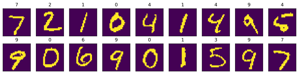
The accuracy is useful mostly as a sanity check: on images, the conditional-independence assumption leaves visible performance on the table.

def predict(X):
    return [bayes_pred_stable(x).argmax(dim=0).type(torch.int32).item()
            for x in X]

X = torch.stack([mnist_test[i][0] for i in range(18)], dim=0)
y = torch.tensor([mnist_test[i][1] for i in range(18)])
preds = predict(X)
d2l.show_images(X, 2, 9, titles=[str(d) for d in preds]);

X = torch.stack([mnist_test[i][0] for i in range(len(mnist_test))], dim=0)
y = torch.tensor([mnist_test[i][1] for i in range(len(mnist_test))])
preds = torch.tensor(predict(X), dtype=torch.int32)
float((preds == y).sum()) / len(y)  # Validation accuracy

0.8427

Recap

• Bayes rule + conditional independence = naive Bayes.
• Training is one pass over the data — count and smooth.
• Surprisingly competitive baseline for text classification (sparse features, large vocab).
• Bad on images (independence is too wrong) — but a great teaching example for Bayesian classification.