Dot products and angles

Geometry and Linear Algebraic Operations

Geometry of Linear Algebra

The geometric intuitions behind the linear algebra used throughout the book. Two viewpoints on a vector \mathbf{v}:

• A position — a point in space.
• A direction — an arrow from the origin.

Most of deep learning works in the second view. From it we get dot products (similarity), angles, projections, hyperplanes (decision boundaries), and determinants (volume changes).

Vectors as geometry

The same array can name a point or a displacement. Deep learning mostly uses the displacement view: directions, lengths, and angles.

v = [1, 7, 0, 1]

\mathbf{u}^\top \mathbf{v} = \|\mathbf{u}\| \|\mathbf{v}\| \cos\theta. Cosine similarity = normalized dot product. The metric behind kernel methods, attention, and contrastive learning:

%matplotlib inline
from d2l import torch as d2l
from IPython import display
import torch
from torchvision import transforms
import torchvision

def angle(v, w):
    return torch.acos(v.dot(w) / (torch.norm(v) * torch.norm(w)))

angle(torch.tensor([0, 1, 2], dtype=torch.float32), torch.tensor([2.0, 3, 4]))

tensor(0.4190)

Hyperplanes as classifiers

A hyperplane is the set \{\mathbf{x} : \mathbf{w}^\top \mathbf{x} = b\}. Linear classifiers split space with one — sign of the dot product gives the prediction. Most of deep learning is “learn good features so a hyperplane works”:

# Load in the dataset
trans = []
trans.append(transforms.ToTensor())
trans = transforms.Compose(trans)
train = torchvision.datasets.FashionMNIST(root="../data", transform=trans,
                                          train=True, download=True)
test = torchvision.datasets.FashionMNIST(root="../data", transform=trans,
                                         train=False, download=True)

X_train_0 = torch.stack(
    [x[0] * 256 for x in train if x[1] == 0]).type(torch.float32)
X_train_1 = torch.stack(
    [x[0] * 256 for x in train if x[1] == 1]).type(torch.float32)
X_test = torch.stack(
    [x[0] * 256 for x in test if x[1] == 0 or x[1] == 1]).type(torch.float32)
y_test = torch.stack([torch.tensor(x[1]) for x in test
                      if x[1] == 0 or x[1] == 1]).type(torch.float32)

# Compute averages
ave_0 = torch.mean(X_train_0, axis=0)
ave_1 = torch.mean(X_train_1, axis=0)

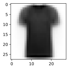
# Plot average t-shirt
d2l.set_figsize()
d2l.plt.imshow(ave_0.reshape(28, 28).tolist(), cmap='Greys')
d2l.plt.show()

Hyperplanes (cont.)

Changing \mathbf{w} rotates the boundary; changing b shifts it. Normalized distance to the boundary is a margin.

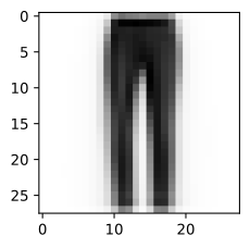
# Plot average trousers
d2l.plt.imshow(ave_1.reshape(28, 28).tolist(), cmap='Greys')
d2l.plt.show()

# Print test set accuracy with eyeballed threshold
w = ave_1 - ave_0
# '@' is Matrix Multiplication operator in pytorch.
predictions = X_test.reshape(2000, -1) @ (w.flatten()) > -1500000

# Accuracy
torch.mean((predictions.type(y_test.dtype) == y_test).float(), dtype=torch.float64)

tensor(0.8730, dtype=torch.float64)

Invertibility and determinant

Square matrices are invertible iff they don’t collapse volumes. The determinant measures the signed volume scale factor:

M = torch.tensor([[1, 2], [1, 4]], dtype=torch.float32)
M_inv = torch.tensor([[2, -1], [-0.5, 0.5]])
M_inv @ M

tensor([[1., 0.],
        [0., 1.]])

torch.det(torch.tensor([[1, -1], [2, 3]], dtype=torch.float32))

tensor(5.)

In code

Translate all of this into NumPy / PyTorch:

# Define tensors
B = torch.tensor([[[1, 2, 3], [4, 5, 6]], [[7, 8, 9], [10, 11, 12]]])
A = torch.tensor([[1, 2], [3, 4]])
v = torch.tensor([1, 2])

# Print out the shapes
A.shape, B.shape, v.shape

(torch.Size([2, 2]), torch.Size([2, 2, 3]), torch.Size([2]))

# Reimplement matrix multiplication
torch.einsum("ij, j -> i", A, v), A@v

(tensor([ 5, 11]), tensor([ 5, 11]))

In code (cont.)

These final snippets connect the geometric ideas to the actual linear-algebra APIs for norms, determinants, and inverses.

torch.einsum("ijk, il, j -> kl", B, A, v)

tensor([[ 90, 126],
        [102, 144],
        [114, 162]])

torch.einsum(B, [0, 1, 2], A, [0, 3], v, [1], [2, 3])

tensor([[ 90, 126],
        [102, 144],
        [114, 162]])

Recap

• Vectors as directions; dot products = cosine similarity; matrices = linear maps; determinant = volume scale.
• Hyperplanes are the decision-boundary primitive of every linear classifier and every linear layer.
• These geometric pictures keep being useful all the way up to attention and high-dim embeddings.