Eigendecompositions

Eigenvectors and Dynamics

A square matrix \mathbf{A} has eigenvalue \lambda and eigenvector \mathbf{v} when

\mathbf{A}\mathbf{v} = \lambda \mathbf{v}.

Geometrically: \mathbf{A} stretches \mathbf{v} by \lambda but doesn’t rotate it. If \mathbf{A} is diagonalizable: \mathbf{A} = \mathbf{V}\mathbf{\Lambda}\mathbf{V}^{-1} — a basis change in which the action is just stretching along axes.

Why we care: matrix powers \mathbf{A}^t are governed by \lambda^t. Repeated application of \mathbf{A} aligns arbitrary inputs with the dominant eigenvector. That’s the heart of vanishing/exploding gradients in RNNs, of PageRank, and of every iterative solver.

A concrete example

Use a small matrix so the geometry is visible: applying \mathbf{A} to an eigenvector changes scale but not direction.

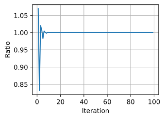
%matplotlib inline
from d2l import torch as d2l
from IPython import display
import torch

torch.linalg.eig(torch.tensor([[2, 1], [2, 3]], dtype=torch.float64))

torch.return_types.linalg_eig(
eigenvalues=tensor([1.+0.j, 4.+0.j], dtype=torch.complex128),
eigenvectors=tensor([[-0.7071+0.j, -0.4472+0.j],
        [ 0.7071+0.j, -0.8944+0.j]], dtype=torch.complex128))

Gershgorin circles

Cheap eigenvalue bounds without computing them: eigenvalues lie in the union of disks centered at a_{ii} with radius \sum_{j \ne i} |a_{ij}|. Useful for stability arguments:

A = torch.tensor([[1.0, 0.1, 0.1, 0.1],
              [0.1, 3.0, 0.2, 0.3],
              [0.1, 0.2, 5.0, 0.5],
              [0.1, 0.3, 0.5, 9.0]])

v, _ = torch.linalg.eig(A)
v

tensor([9.0803+0.j, 0.9923+0.j, 4.9539+0.j, 2.9734+0.j])

Eigenvectors govern long-run behavior

Power iteration: keep multiplying by \mathbf{A}. The direction converges to the leading eigenvector; the norm grows like \lambda_1^t:

torch.manual_seed(42)

k = 5
A = torch.randn(k, k, dtype=torch.float64)
A

tensor([[ 0.2996,  0.2424,  0.2832, -0.2329,  0.6712],
        [ 0.7818, -1.7903, -1.7484,  0.1735, -0.1182],
        [-1.7446, -0.4695,  0.4573,  0.5177, -0.2771],
        [-0.6641,  0.6551,  0.2616, -1.5265, -0.3311],
        [-0.6378,  0.1072,  0.7096,  0.3009, -0.2869]], dtype=torch.float64)

# Calculate the sequence of norms after repeatedly applying `A`
v_in = torch.randn(k, 1, dtype=torch.float64)

norm_list = [torch.norm(v_in).item()]
for i in range(1, 100):
    v_in = A @ v_in
    norm_list.append(torch.norm(v_in).item())

d2l.plot(torch.arange(0, 100), norm_list, 'Iteration', 'Value')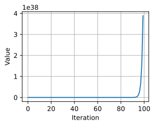

# Compute the scaling factor of the norms
norm_ratio_list = []
for i in range(1, 100):
    norm_ratio_list.append(norm_list[i]/norm_list[i - 1])

d2l.plot(torch.arange(1, 100), norm_ratio_list, 'Iteration', 'Ratio')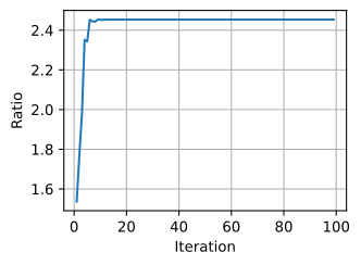

Relating back

After repeated multiplication, normalize the vector to read off the direction; the scale factor estimates the dominant eigenvalue.

# Compute the eigenvalues
eigs = torch.linalg.eig(A).eigenvalues.tolist()
norm_eigs = [torch.abs(torch.tensor(x)) for x in eigs]
norm_eigs.sort()
print(f'norms of eigenvalues: {norm_eigs}')

norms of eigenvalues: [tensor(0.3490), tensor(1.1296), tensor(1.1296), tensor(1.1828), tensor(2.4532)]

# Rescale the matrix `A`
A /= norm_eigs[-1]

# Do the same experiment again
v_in = torch.randn(k, 1, dtype=torch.float64)

norm_list = [torch.norm(v_in).item()]
for i in range(1, 100):
    v_in = A @ v_in
    norm_list.append(torch.norm(v_in).item())

d2l.plot(torch.arange(0, 100), norm_list, 'Iteration', 'Value')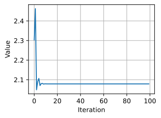

# Also plot the ratio
norm_ratio_list = []
for i in range(1, 100):
    norm_ratio_list.append(norm_list[i]/norm_list[i-1])

d2l.plot(torch.arange(1, 100), norm_ratio_list, 'Iteration', 'Ratio')

Recap

• \mathbf{A}\mathbf{v} = \lambda \mathbf{v}: \mathbf{A} acts as scaling along the eigenvector axes.
• Largest |\lambda| controls long-run iterated dynamics.
• Symmetric matrices have orthonormal eigenvectors and real eigenvalues — the basis for PCA.
• Vanishing/exploding RNN gradients = “iterated map” with bad spectral radius.