Bernoulli

Distributions

Common Probability Distributions

A reference tour of the distributions used throughout the book — what they look like, when they apply, and how to sample / evaluate them in code.

• Bernoulli — single coin flip; binary classification conditional.
• Discrete uniform — equiprobable categories.
• Continuous uniform — random initialization, dropout masks (in expectation).
• Binomial — count of successes in n Bernoullis.
• Poisson — rare events count; CTR distributions, click counts.
• Gaussian — by far the most-used; CLT, regression noise model, default prior.

Setup

Imports and plotting helpers are shared across the PMF, PDF, CDF, and sampling examples below.

%matplotlib inline
from d2l import torch as d2l
from IPython import display
from math import erf, factorial
import torch

torch.pi = torch.acos(torch.zeros(1)) * 2  # Define pi in torch

P(X=1) = p, P(X=0) = 1-p. Mean p, variance p(1-p):

p = 0.3

d2l.set_figsize()
d2l.plt.stem([0, 1], [1 - p, p])
d2l.plt.xlabel('x')
d2l.plt.ylabel('p.m.f.')
d2l.plt.show()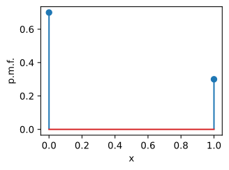

x = torch.arange(-1, 2, 0.01)

def F(x):
    return 0 if x < 0 else 1 if x > 1 else 1 - p

d2l.plot(x, torch.tensor([F(y) for y in x]), 'x', 'c.d.f.')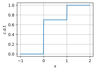

1*(torch.rand(10, 10) < p)

tensor([[0, 1, 0, 0, 0, 0, 1, 1, 1, 1],
        [1, 1, 0, 0, 0, 0, 0, 1, 0, 0],
        [1, 0, 0, 0, 0, 0, 0, 1, 0, 0],
        [1, 0, 0, 1, 0, 1, 0, 0, 1, 1],
        [0, 0, 1, 0, 1, 1, 0, 0, 0, 0],
        [0, 0, 0, 1, 0, 0, 0, 0, 1, 0],
        [0, 1, 0, 0, 0, 0, 0, 0, 0, 0],
        [0, 0, 1, 0, 0, 1, 0, 0, 0, 0],
        [0, 0, 0, 0, 0, 0, 0, 0, 1, 1],
        [0, 0, 1, 0, 0, 0, 0, 0, 1, 0]])

Discrete uniform

Equally likely categories. Maximum entropy on a finite set with no prior knowledge:

n = 5

d2l.plt.stem([i+1 for i in range(n)], n*[1 / n])
d2l.plt.xlabel('x')
d2l.plt.ylabel('p.m.f.')
d2l.plt.show()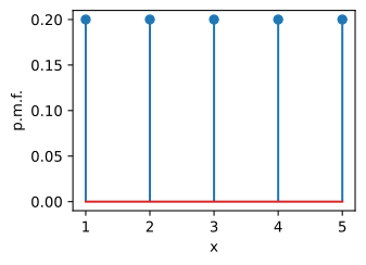

x = torch.arange(-1, 6, 0.01)

def F(x):
    return 0 if x < 1 else 1 if x > n else torch.floor(x) / n

d2l.plot(x, torch.tensor([F(y) for y in x]), 'x', 'c.d.f.')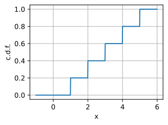

torch.randint(1, n, size=(10, 10))

tensor([[1, 3, 3, 3, 4, 1, 3, 4, 3, 2],
        [1, 3, 2, 4, 3, 2, 1, 4, 4, 2],
        [3, 1, 2, 3, 3, 4, 1, 2, 4, 4],
        [4, 4, 2, 4, 4, 3, 3, 1, 4, 1],
        [3, 4, 1, 1, 4, 4, 2, 3, 3, 3],
        [3, 2, 4, 3, 3, 4, 3, 4, 2, 2],
        [4, 3, 4, 3, 4, 1, 1, 2, 1, 1],
        [2, 2, 3, 2, 2, 3, 3, 4, 1, 1],
        [2, 3, 4, 2, 2, 3, 2, 2, 2, 4],
        [3, 2, 1, 3, 1, 4, 4, 4, 4, 1]])

Continuous uniform

Density \frac{1}{b-a} on [a, b]. Source of pseudo-random samples for Monte Carlo and dropout:

a, b = 1, 3

x = torch.arange(0, 4, 0.01)
p = (x > a).type(torch.float32)*(x < b).type(torch.float32)/(b-a)
d2l.plot(x, p, 'x', 'p.d.f.')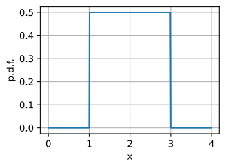

def F(x):
    return 0 if x < a else 1 if x > b else (x - a) / (b - a)

d2l.plot(x, torch.tensor([F(y) for y in x]), 'x', 'c.d.f.')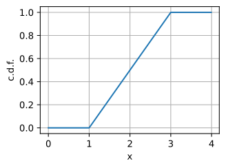

(b - a) * torch.rand(10, 10) + a

tensor([[1.2243, 1.1095, 2.8709, 1.1908, 2.5147, 1.6325, 1.8333, 2.7934, 2.6653,
         1.8213],
        [2.9245, 1.0105, 2.0162, 1.8633, 2.6736, 2.4816, 2.2687, 2.0998, 2.4288,
         1.0970],
        [1.7825, 1.5883, 2.7182, 2.6172, 1.9619, 1.8157, 2.6660, 2.1698, 1.3037,
         1.1473],
...
        [2.2590, 1.1515, 2.8519, 2.9638, 1.7060, 1.3417, 1.6249, 2.3621, 1.9515,
         2.4415],
        [2.6999, 1.3334, 2.5928, 1.2432, 1.2504, 2.3189, 1.4276, 2.5106, 2.4501,
         1.2251],
        [1.7683, 2.9988, 2.2427, 2.5229, 1.2951, 1.8569, 1.0759, 2.3962, 1.9412,
         1.2245]])

Binomial

Sum of n iid Bernoullis. Bell-shaped for large n (Gaussian limit):

n, p = 10, 0.2

# Compute binomial coefficient
def binom(n, k):
    comb = 1
    for i in range(min(k, n - k)):
        comb = comb * (n - i) // (i + 1)
    return comb

pmf = d2l.tensor([p**i * (1-p)**(n - i) * binom(n, i) for i in range(n + 1)])

d2l.plt.stem([i for i in range(n + 1)], pmf)
d2l.plt.xlabel('x')
d2l.plt.ylabel('p.m.f.')
d2l.plt.show()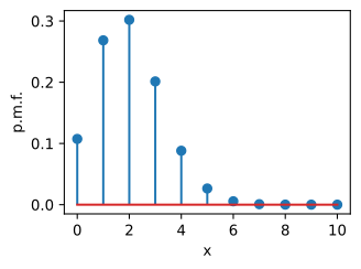

x = torch.arange(-1, 11, 0.01)
cmf = torch.cumsum(pmf, dim=0)

def F(x):
    return 0 if x < 0 else 1 if x > n else cmf[int(x)]

d2l.plot(x, torch.tensor([F(y) for y in x.tolist()]), 'x', 'c.d.f.')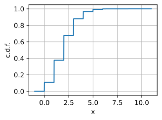

m = torch.distributions.binomial.Binomial(n, p)
m.sample(sample_shape=(10, 10))

tensor([[4., 2., 4., 3., 5., 2., 3., 2., 2., 2.],
        [1., 1., 1., 1., 2., 3., 1., 2., 1., 5.],
        [1., 4., 0., 0., 1., 4., 2., 2., 1., 2.],
        [3., 1., 5., 2., 3., 1., 2., 3., 3., 2.],
        [3., 1., 3., 0., 1., 5., 2., 0., 2., 1.],
        [1., 0., 5., 2., 3., 2., 2., 2., 3., 4.],
        [2., 1., 3., 2., 1., 3., 1., 3., 4., 2.],
        [2., 1., 3., 0., 3., 3., 3., 1., 3., 1.],
        [1., 2., 2., 3., 2., 0., 3., 2., 4., 2.],
        [2., 2., 3., 5., 2., 2., 1., 1., 1., 2.]])

Poisson

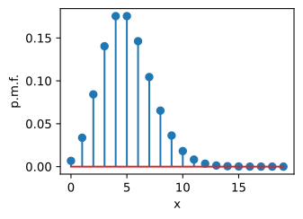
Rare events: P(X = k) = \frac{\lambda^k e^{-\lambda}}{k!}. Approximates binomial with n large, p small, np \to \lambda:

Poisson CDF

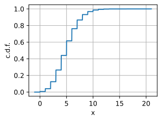
The cumulative distribution sums the probability of observing up to k events:

F(k)=P(X \le k).

Poisson samples

Sampling turns the distribution into count data: nonnegative integers with mean and variance both near \lambda.

tensor([[ 5.,  5.,  6.,  5.,  5.,  8.,  7.,  6.,  8.,  8.],
        [ 9.,  4.,  0.,  7.,  8.,  1.,  4.,  8.,  5.,  5.],
        [ 5.,  4.,  1.,  5.,  7.,  6.,  2.,  5.,  3.,  9.],
        [ 6.,  8.,  6.,  6.,  9.,  7.,  3.,  1.,  4.,  2.],
        [ 8., 11.,  4.,  5.,  3.,  2.,  2.,  3.,  7.,  2.],
        [ 7., 10.,  7.,  4.,  2.,  4.,  4.,  7.,  8.,  4.],
        [ 5.,  7.,  6.,  7.,  5.,  2.,  2.,  5.,  5.,  7.],
        [ 7.,  2.,  8.,  6.,  5.,  6.,  5.,  4.,  5.,  5.],
        [ 2.,  7.,  8.,  2.,  5.,  3.,  5.,  4.,  6.,  7.],
        [ 7.,  4.,  6.,  8.,  9.,  5.,  3.,  5.,  5.,  3.]])

Gaussian

\mathcal{N}(\mu, \sigma^2) — bell curve. CLT makes it the limit of many small contributions; that’s why it’s everywhere:

p = 0.2
ns = [1, 10, 100, 1000]
d2l.plt.figure(figsize=(10, 3))
for i in range(4):
    n = ns[i]
    pmf = torch.tensor([p**i * (1-p)**(n-i) * binom(n, i)
                        for i in range(n + 1)])
    d2l.plt.subplot(1, 4, i + 1)
    d2l.plt.stem([(i - n*p)/torch.sqrt(torch.tensor(n*p*(1 - p)))
                  for i in range(n + 1)], pmf)
    d2l.plt.xlim([-4, 4])
    d2l.plt.xlabel('x')
    d2l.plt.ylabel('p.m.f.')
    d2l.plt.title("n = {}".format(n))
d2l.plt.show()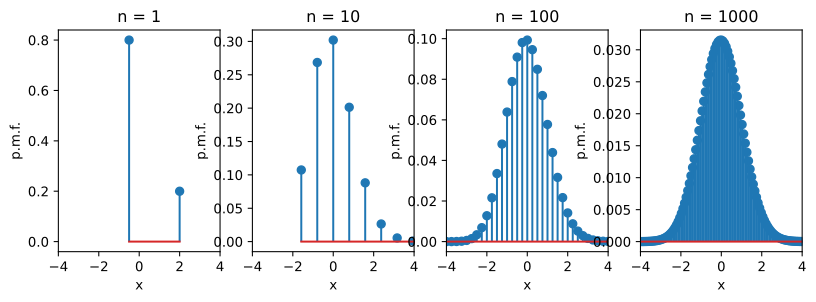

mu, sigma = 0, 1

x = torch.arange(-3, 3, 0.01)
p = 1 / torch.sqrt(2 * torch.pi * sigma**2) * torch.exp(
    -(x - mu)**2 / (2 * sigma**2))

d2l.plot(x, p, 'x', 'p.d.f.')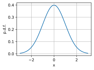

Gaussian (cont.)

Changing \mu shifts the bell curve; changing \sigma spreads it. Samples concentrate near the mean and thin out in the tails.

def phi(x):
    return (1.0 + erf((x - mu) / (sigma * torch.sqrt(d2l.tensor(2.))))) / 2.0

d2l.plot(x, torch.tensor([phi(y) for y in x.tolist()]), 'x', 'c.d.f.')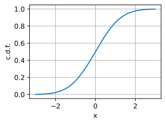

torch.normal(mu, sigma, size=(10, 10))

tensor([[-1.0753, -0.2009,  1.2762, -1.4277, -0.7739,  0.7547,  1.3835, -0.8503,
          1.2070, -0.7471],
        [ 0.6481,  0.2798,  1.1094,  1.4962, -1.5071, -2.6643,  0.4088,  0.2013,
         -1.0790,  0.1552],
        [ 0.0058,  0.5766, -1.0608,  0.5905, -0.0917,  0.5187, -1.1351,  1.1590,
         -1.1337, -0.1141],
...
        [-0.4446, -1.2968,  0.2200, -1.7508,  0.0626, -1.3804,  2.4323,  0.2062,
         -1.0654, -0.8014],
        [-0.3614,  0.6907,  1.2591,  0.0988,  1.3787,  0.6183,  2.7467,  1.5583,
          0.6596, -1.4697],
        [ 0.7863,  0.7149,  0.2460,  2.2550, -0.2982, -1.5202, -0.2899,  0.1406,
          1.5426,  1.5907]])

Recap

• A small toolkit covers most needs: Bernoulli, uniform (discrete/continuous), binomial, Poisson, Gaussian.
• CLT makes the Gaussian central — sums of many small effects look Gaussian.
• Each distribution has a closed-form NLL → standard loss in DL.