Stacking from scratch

Deep Recurrent Neural Networks

Deep RNNs

A single RNN layer is already deep in time — but within one time step, input-to-output is just one nonlinearity.

Stacking RNN layers makes the model deep along the layer axis too. Each layer sees the previous layer’s hidden states as its input sequence; topmost layer feeds the readout.

\mathbf{H}_t^{(l)} = \phi_l(\mathbf{H}_t^{(l-1)} \mathbf{W}_{xh}^{(l)} + \mathbf{H}_{t-1}^{(l)} \mathbf{W}_{hh}^{(l)} + \mathbf{b}_h^{(l)}).

Typical sizes: width 64–2048, depth 1–8.

Architecture

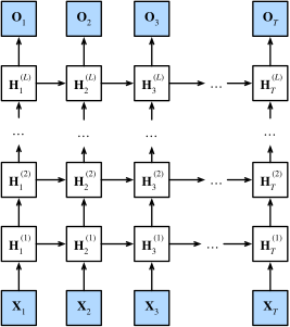
Layer l at time t depends on layer l at time t{-}1 and layer l{-}1 at time t.

Setup

from d2l import mxnet as d2l
from mxnet import np, npx
from mxnet.gluon import rnn
npx.set_np()

A StackedRNNScratch is just a list of RNNScratch cells — each layer’s input width is num_hiddens (except the bottom layer, which sees raw inputs):

class StackedRNNScratch(d2l.Module):
    def __init__(self, num_inputs, num_hiddens, num_layers, sigma=0.01):
        super().__init__()
        self.save_hyperparameters()
        self.rnns = [d2l.RNNScratch(num_inputs if i==0 else num_hiddens,
                                    num_hiddens, sigma)
                     for i in range(num_layers)]

The forward pass walks the layers, feeding each layer’s output sequence into the next:

def forward(self, inputs, Hs=None):
    outputs = inputs
    if Hs is None: Hs = [None] * self.num_layers
    for i in range(self.num_layers):
        outputs, Hs[i] = self.rnns[i](outputs, Hs[i])
        if i < self.num_layers - 1:
            outputs = d2l.stack(outputs, 0)
    return outputs, Hs

Training the stacked RNN

Two-layer stack on The Time Machine. Lower learning rate (lr=2) — deeper recurrents are harder to optimize:

data = d2l.TimeMachine(batch_size=1024, num_steps=32)
rnn_block = StackedRNNScratch(num_inputs=len(data.vocab),
                              num_hiddens=32, num_layers=2)
model = d2l.RNNLMScratch(rnn_block, vocab_size=len(data.vocab), lr=2)
trainer = d2l.Trainer(max_epochs=100, gradient_clip_val=1, num_gpus=1)
trainer.fit(model, data)

Concise: multilayer GRU

nn.GRU(..., num_layers=L, dropout=p) collapses the stack into one library call — and adds dropout between layers, which is the standard regularizer for stacked RNNs:

class GRU(d2l.RNN):
    """The multilayer GRU model."""
    def __init__(self, num_hiddens, num_layers, dropout=0):
        d2l.Module.__init__(self)
        self.save_hyperparameters()
        self.rnn = rnn.GRU(num_hiddens, num_layers, dropout=dropout)

Training and decoding

Two-layer GRU LM, same Trainer:

gru = GRU(num_hiddens=32, num_layers=2)
model = d2l.RNNLM(gru, vocab_size=len(data.vocab), lr=2)
trainer.fit(model, data)
model.predict('it has', 20, data.vocab, d2l.try_gpu())

Decode from a prefix:

Recap

• Deep RNNs stack L recurrent layers; layer l’s input is layer l{-}1’s output sequence.
• Same idea applies to vanilla RNN, LSTM, or GRU cells.
• Use lower learning rate and (usually) inter-layer dropout — vertical depth makes optimization noticeably trickier.
• nn.GRU(..., num_layers=L, dropout=p) is the production one-liner.