%matplotlib inline
from d2l import mxnet as d2l
from mpl_toolkits import mplot3d
from mxnet import np, npx
npx.set_np()Convex sets and functions
Why Convexity Matters
Deep learning loss surfaces are not convex. So why a chapter on convexity? Two reasons:
- It’s the only setting where we can prove convergence of algorithms cleanly. Pre-deep-learning optimization theory is almost entirely about convex problems.
- Local behavior near a deep-learning minimum often looks approximately convex. Many practical tricks (averaging, Polyak averaging, weight averaging like SWA) are motivated by convex theory.
If a method fails on a convex problem, it has no hope on a non-convex one.
A set \mathcal{X} is convex if for all x, x' \in \mathcal{X} and \lambda \in [0, 1], \lambda x + (1-\lambda) x' \in \mathcal{X} — it contains every line segment between its points.
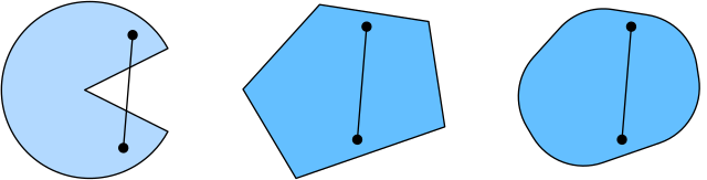
Nonconvex (left) vs. convex (middle, right).
A function f is convex if for all such x, x', \lambda:
\lambda f(x) + (1-\lambda) f(x') \;\geq\; f(\lambda x + (1-\lambda) x').
The chord lies above the function:
f = lambda x: 0.5 * x**2  # Convex
g = lambda x: d2l.cos(np.pi * x)  # Nonconvex
h = lambda x: d2l.exp(0.5 * x)  # Convex

x, segment = d2l.arange(-2, 2, 0.01), d2l.tensor([-1.5, 1])
d2l.use_svg_display()
_, axes = d2l.plt.subplots(1, 3, figsize=(9, 3))
for ax, func in zip(axes, [f, g, h]):
    d2l.plot([x, segment], [func(x), func(segment)], axes=ax)
Convex set algebra
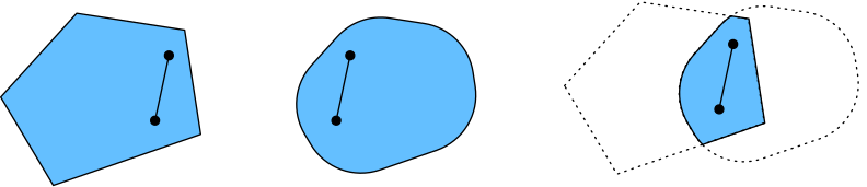
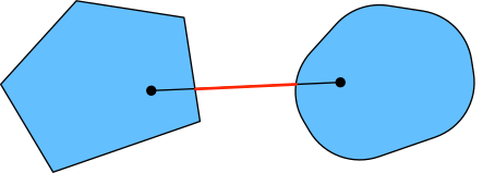
Intersections of convex sets are convex (useful: feasible sets defined by multiple convex constraints stay convex). Unions are not.
Constrained convex optimization
For constrained problems \min f(x) s.t. c_i(x) \le 0, three workhorse techniques:
- Lagrangian — turn constraints into penalty terms with multipliers \alpha_i \ge 0.
- Penalty methods — soft constraints via large \sum_i \max(0, c_i(x))^2 terms.
- Projection — after each gradient step, project back onto the feasible set.
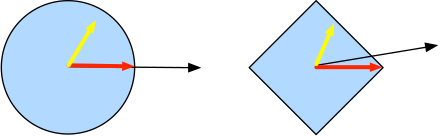
Projecting an external point onto a convex set.