1D convolution

Sentiment Analysis: Using Convolutional Neural Networks

textCNN

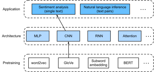
textCNN (Kim, 2014) — a 1D conv net for sentiment. Different architecture, same task as the RNN deck.

Why CNNs on text? Each filter is a learned n-gram detector. Run several filter widths in parallel (3, 4, 5 words) for multi-scale coverage. Max-over-time pool collapses position; concat → linear → softmax. Fast, strong, parallelizable.

Pipeline

GloVe → 1D conv filters of varying widths → max-pool → classifier.

Setup

from d2l import mxnet as d2l
from mxnet import gluon, init, np, npx
from mxnet.gluon import nn
npx.set_np()

batch_size = 64
train_iter, test_iter, vocab = d2l.load_data_imdb(batch_size)

Sliding kernel over a 1D sequence. Output element = elementwise multiply + sum of an n-token window:

1D conv: kernel (1, 2) slides over input; first output is 0 \cdot 1 + 1 \cdot 2 = 2.

def corr1d(X, K):
    w = K.shape[0]
    Y = d2l.zeros((X.shape[0] - w + 1))
    for i in range(Y.shape[0]):
        Y[i] = (X[i: i + w] * K).sum()
    return Y

Multi-channel 1D conv

Embedding dim = input channels. Kernel has the same channel count; output is single-channel (or multi if you have multiple kernels).

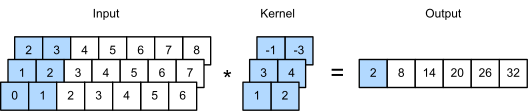
3-channel 1D conv.

X, K = d2l.tensor([0, 1, 2, 3, 4, 5, 6]), d2l.tensor([1, 2])
corr1d(X, K)

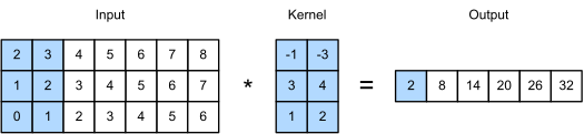
Equivalent 2D-conv view

Equivalent to a 2D conv with kernel height = input height:

def corr1d_multi_in(X, K):
    # First, iterate through the 0th dimension (channel dimension) of `X` and
    # `K`. Then, add them together
    return sum(corr1d(x, k) for x, k in zip(X, K))

X = d2l.tensor([[0, 1, 2, 3, 4, 5, 6],
              [1, 2, 3, 4, 5, 6, 7],
              [2, 3, 4, 5, 6, 7, 8]])
K = d2l.tensor([[1, 2], [3, 4], [-1, -3]])
corr1d_multi_in(X, K)

Max-over-time pooling

Take the max over the time axis for each filter. Resulting feature is independent of where in the sequence the n-gram appeared. One scalar per filter, regardless of sentence length:

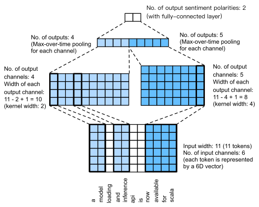
Max-over-time = max along the sequence axis.

textCNN model

Embedding (frozen GloVe + a fine-tunable copy) → parallel 1D convs at widths 3, 4, 5 → max-over-time → concat → dropout → linear:

class TextCNN(nn.Block):
    def __init__(self, vocab_size, embed_size, kernel_sizes, num_channels):
        super().__init__()
        self.embedding = nn.Embedding(vocab_size, embed_size)
        # The embedding layer not to be trained
        self.constant_embedding = nn.Embedding(vocab_size, embed_size)
        self.dropout = nn.Dropout(0.5)
        self.decoder = nn.Dense(2)
        # The max-over-time pooling layer has no parameters, so this instance
        # can be shared
        self.pool = nn.GlobalMaxPool1D()
        # Create multiple one-dimensional convolutional layers
        self.convs = nn.Sequential()
        for c, k in zip(num_channels, kernel_sizes):
            self.convs.add(nn.Conv1D(c, k, activation='relu'))

    def forward(self, inputs):
        # Concatenate two embedding layer outputs with shape (batch size, no.
        # of tokens, token vector dimension) along vectors
        embeddings = np.concatenate((
            self.embedding(inputs), self.constant_embedding(inputs)), axis=2)
        # Per the input format of one-dimensional convolutional layers,
        # rearrange the tensor so that the second dimension stores channels
        embeddings = embeddings.transpose(0, 2, 1)
        # For each one-dimensional convolutional layer, after max-over-time
        # pooling, a tensor of shape (batch size, no. of channels, 1) is
        # obtained. Remove the last dimension and concatenate along channels
        encoding = np.concatenate([
            np.squeeze(self.pool(conv(embeddings)), axis=-1)
            for conv in self.convs], axis=1)
        outputs = self.decoder(self.dropout(encoding))
        return outputs

textCNN instance

The concrete model uses 100 channels at each kernel width. After max-over-time pooling, the classifier sees sum(num_channels) features, independent of review length.

embed_size, kernel_sizes, nums_channels = 100, [3, 4, 5], [100, 100, 100]
devices = d2l.try_all_gpus()
net = TextCNN(len(vocab), embed_size, kernel_sizes, nums_channels)
net.initialize(init.Xavier(), ctx=devices)

Loading pretrained GloVe

Both embedding tables start from the same GloVe vectors: one stays fixed as a semantic anchor, the other is fine-tuned for sentiment-specific cues.

glove_embedding = d2l.TokenEmbedding('glove.6b.100d')
embeds = glove_embedding[vocab.idx_to_token]
net.embedding.weight.set_data(embeds)
net.constant_embedding.weight.set_data(embeds)
for p in net.constant_embedding.collect_params().values():
    p.grad_req = 'null'

Training

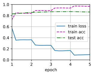
CNNs train fast because all windows are processed in parallel. Use the metric output to compare with the BiLSTM deck: similar accuracy, less sequential computation.

# lr divided by batch_size: gluon Trainer no longer rescales (issue 7 fix in d2l.train_batch_ch13)
lr, num_epochs = 1.5625e-5, 5
trainer = gluon.Trainer(net.collect_params(), 'adam', {'learning_rate': lr})
loss = gluon.loss.SoftmaxCrossEntropyLoss()
d2l.train_ch13(net, train_iter, test_iter, loss, trainer, num_epochs, devices)

d2l.predict_sentiment(net, vocab, 'this movie is so great')

d2l.predict_sentiment(net, vocab, 'this movie is so bad')

Recap

textCNN = parallel 1D convs over word embeddings + max pooling + linear head.
Each filter learns an n-gram detector; different widths give multi-scale coverage.
Comparable accuracy to BiLSTM on IMDb at a fraction of the training time and zero recurrence.
The shape (parallel filter widths, pooled features) is the template for many text-classification CNNs that followed.