Predicting House Prices on Kaggle

House prices: a full ML pipeline

House Prices: Advanced Regression Techniques — predict sale prices of Ames, Iowa houses from 80 numeric and categorical features. A small but realistic end-to-end ML exercise.

What makes it interesting:

  • 1460 train / 1459 test — small data.
  • 80 mixed features — needs preprocessing.
  • Missing values in dozens of columns.
  • Targets vary 10× ($65k–$755k) — wrong loss overweights expensive houses.

The MLP is 5 lines. The lesson is the pipeline around it — preprocessing, the right loss, CV, submission.

Kaggle in 30 seconds

Kaggle hosts open ML competitions. Download train + test CSVs, train locally, upload predictions, get scored on a held-out portion of the test set.

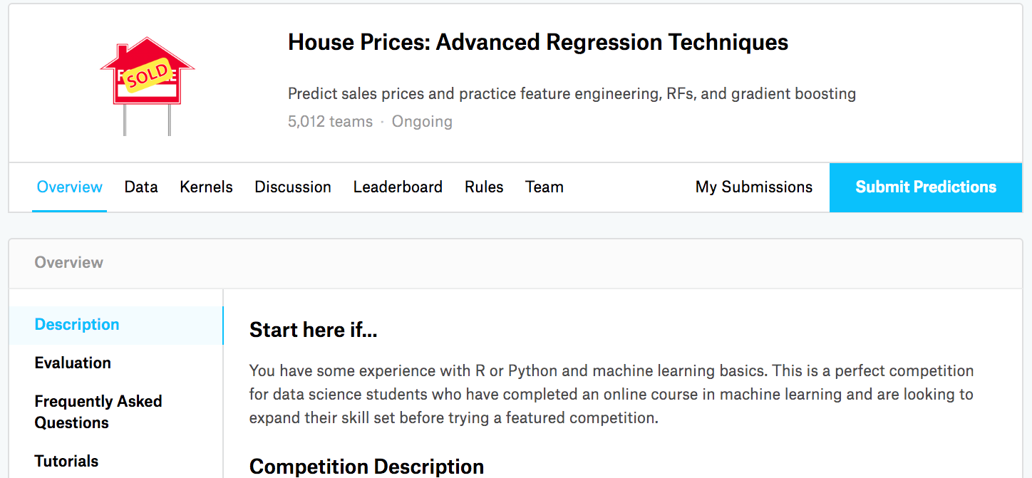
Kaggle competition page.

The House Prices page

The competition’s data tab — download and inspect.

Real-world ML practice: data isn’t preprocessed for you, the leaderboard tells you instantly if you’re better than baseline, and the public/private split keeps people honest about overfitting.

Setup and data download

A reusable hash-checked download helper we’ll keep using throughout the book:

%matplotlib inline
from d2l import mxnet as d2l
from mxnet import gluon, autograd, init, np, npx
from mxnet.gluon import nn
import pandas as pd

npx.set_np()
def download(url, folder, sha1_hash=None):
    """Download a file to folder and return the local filepath."""

def extract(filename, folder):
    """Extract a zip/tar file into folder."""

Reading the data

Wrap train and test CSVs in a KaggleHouse(d2l.DataModule):

class KaggleHouse(d2l.DataModule):
    def __init__(self, batch_size, train=None, val=None):
        super().__init__()
        self.save_hyperparameters()
        if self.train is None:
            self.raw_train = pd.read_csv(d2l.download(
                d2l.DATA_URL + 'kaggle_house_pred_train.csv', self.root,
                sha1_hash='585e9cc93e70b39160e7921475f9bcd7d31219ce'))
            self.raw_val = pd.read_csv(d2l.download(
                d2l.DATA_URL + 'kaggle_house_pred_test.csv', self.root,
                sha1_hash='fa19780a7b011d9b009e8bff8e99922a8ee2eb90'))
data = KaggleHouse(batch_size=64)
print(data.raw_train.shape)
print(data.raw_val.shape)

What the rows look like

print(data.raw_train.iloc[:4, [0, 1, 2, 3, -3, -2, -1]])

Mixed numeric and categorical columns; lots of missing values; final column is the target SalePrice. Models eat tensors, not DataFrames — preprocessing is mandatory.

Three preprocessing transforms

Apply on train + test together so train statistics match what we’ll see at test time:

  1. Numeric NaN → mean. Simple imputation; median or zero are alternatives.
  2. Standardize numeric columns to mean 0, std 1 — makes optimization well-conditioned across wildly different scales.
  3. One-hot encode categorical columns. NaN becomes its own category — missing-as-a-signal.

The transforms in code

def preprocess(self):
    # Remove the ID and label columns
    label = 'SalePrice'
    features = pd.concat(
        (self.raw_train.drop(columns=['Id', label]),
         self.raw_val.drop(columns=['Id'])))
    # Standardize numerical columns using training-set statistics only
    # (to avoid leaking test-set information into the normalization).
    numeric_features = features.select_dtypes(include='number').columns
    n_train = self.raw_train.shape[0]
    train_mean = features[numeric_features].iloc[:n_train].mean()
    train_std = features[numeric_features].iloc[:n_train].std()
    features[numeric_features] = (
        features[numeric_features] - train_mean) / train_std
    # Replace NAN numerical features by 0
    features[numeric_features] = features[numeric_features].fillna(0)
    # Replace discrete features by one-hot encoding
    features = pd.get_dummies(features, dummy_na=True)
    # Save preprocessed features
    self.train = features[:n_train].copy()
    self.train[label] = self.raw_train[label]
    self.val = features[n_train:].copy()
data.preprocess()
data.train.shape

After preprocessing: ~330 columns of well-scaled floats.

Choosing the right loss

Plain squared error penalizes a $10k mistake on a $70k house the same as on a $700k house. The relative error is more honest — predict the logarithm of the price:

\text{RMSLE} = \sqrt{\frac{1}{n} \sum_{i=1}^{n} \big(\log y_i - \log \hat y_i\big)^2}.

The official Kaggle metric for this competition. Mistakes are measured as percentages, not dollars.

Loss in code

def get_dataloader(self, train):
    label = 'SalePrice'
    data = self.train if train else self.val
    if label not in data: return
    get_tensor = lambda x: d2l.tensor(x.values.astype(float),
                                      dtype=d2l.float32)
    # Logarithm of prices 
    tensors = (get_tensor(data.drop(columns=[label])),  # X
               d2l.reshape(d2l.log(get_tensor(data[label])), (-1, 1)))  # Y
    return self.get_tensorloader(tensors, train)

K-fold cross-validation

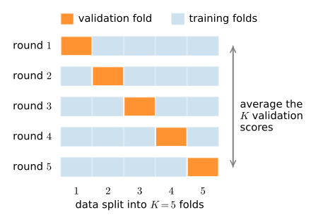
With ~1500 training examples, a single 80/20 split is noisy. K-fold CV: split into K folds, train K times holding each fold out, average the scores.

fold 1:  [ val ][ train ][ train ][ train ][ train ]
fold 2:  [train][  val  ][ train ][ train ][ train ]
fold 3:  [train][ train ][  val  ][ train ][ train ]
fold 4:  [train][ train ][ train ][  val  ][ train ]
fold 5:  [train][ train ][ train ][ train ][  val  ]

Costs K\times more compute; gives a stable estimate of generalization error.

K-fold in code

def k_fold_data(data, k):
    rets = []
    fold_size = data.train.shape[0] // k
    for j in range(k):
        idx = list(range(j * fold_size, (j+1) * fold_size))
        rets.append(KaggleHouse(data.batch_size,
                                data.train.drop(index=idx),
                                data.train.iloc[idx]))
    return rets
def k_fold(trainer, data, k, lr):
    val_loss, models = [], []
    for i, data_fold in enumerate(k_fold_data(data, k)):
        model = d2l.LinearRegression(lr)
        model.board.yscale='log'
        if i != 0: model.board.display = False
        trainer.fit(model, data_fold)
        val_loss.append(float(model.board.data['val_loss'][-1].y))
        models.append(model)
    print(f'average validation log mse = {sum(val_loss)/len(val_loss)}')
    return models

Model selection

trainer = d2l.Trainer(max_epochs=10)
models = k_fold(trainer, data, k=5, lr=0.01)

In practice you’d grid- or random-search over learning rate, hidden size, weight decay, dropout. Same loop, different hyperparameters. Pick the config with the lowest average val score.

Submitting predictions

Final step: re-fit on all training data (no validation hold-out), predict the test set, write the Kaggle-format CSV:

preds = [model(d2l.tensor(data.val.values.astype(float), dtype=d2l.float32))
         for model in models]
# Taking exponentiation of predictions in the logarithm scale
ensemble_preds = d2l.reduce_mean(d2l.exp(d2l.concat(preds, 1)), 1)
submission = pd.DataFrame({'Id':data.raw_val.Id,
                           'SalePrice':d2l.numpy(ensemble_preds)})
submission.to_csv('submission.csv', index=False)
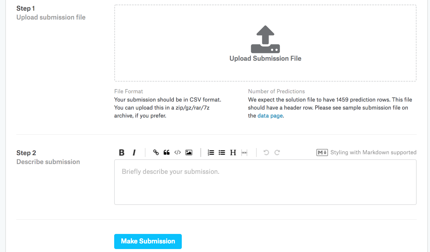
Upload the CSV; Kaggle scores it instantly against the held-out half of the test set.

The general competition recipe

Same shape works for almost any tabular ML competition:

  1. Download train + test data.
  2. Preprocess — impute, scale, encode (combined stats).
  3. Choose the right loss — match the scoring metric.
  4. K-fold CV for generalization estimate + HP search.
  5. Refit on all training data with the best HPs.
  6. Submit predictions in the host’s format.

GBDTs (XGBoost / LightGBM) usually win tabular; nets shine on images, text, audio. The pipeline is the same.

Recap

  • Real-world ML is mostly pipeline, not model architecture.
  • Heterogeneous tabular data → impute, standardize, one-hot encode.
  • Match the loss to the metric — log-RMSE for prices, not squared error.
  • K-fold CV for stable generalization estimates on small data.
  • Refit on full data before final predictions.
  • The MLP is a few lines; everything around it is the lesson.