Dive into Deep Learning · §4.5
Why over-parametrized networks generalize
double descent · the optimizer as regularizer · grokking.
Motivation
Fitting the training data is only the intermediate step. The real quest is to find patterns that predict well on unseen data.
01
Overfitting, revisited
inductive bias and the interpolation regime
Overfitting
No algorithm generalizes better on all distributions. Given finite data, a model must lean on inductive biases that prefer some solutions over others.
The generalization gap is the difference between test and training error. A large gap means we have overfit.
Classical recipe to close the gap: make the model less complex.
Overfitting
Modern networks can be expressive enough to fit large training sets and even random labels.
So the classical levers behave strangely:
Worst-case bounds based on the complete hypothesis class are often vacuous at modern scales. Data- and algorithm-dependent explanations remain active work.
02
Double descent
the U-curve, and what lies past it
Double descent
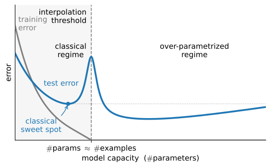
Classical theory predicts a U-shaped test-error curve as capacity grows:
\underbrace{\text{error}}_{\text{test}} \;=\; \underbrace{\text{bias}^2}_{\downarrow\ \text{with capacity}} \;+\; \underbrace{\text{variance}}_{\uparrow\ \text{with capacity}}.
Too little capacity underfits; too much overfits; a sweet spot sits in between.
This is the left half of the picture on the next slide, and it is all the classical story predicts.
One curve, two regimes: the classical U ends at the interpolation threshold, where training error reaches zero and test error peaks — then descends a second time. That second descent is contingent on the model, data, optimizer, and training budget.
Double descent
In linear least-squares and random-feature models, the minimum-norm interpolant can have high variance near a rank transition.
Past that transition, additional features create more interpolating solutions, and the minimum-norm solution can have lower variance.
The appendix (the concentration-and-generalization section) derives this mechanism in a specified model. It is not a theorem that every deep network follows the same curve or selects the same kind of interpolant.
Double descent
Model size is only one of three ways to cross the threshold (Nakkiran et al., 2021):
Nakkiran et al. propose effective model complexity, how many examples the full training procedure (model, optimizer, and budget) can fit. It organizes their observed model-, epoch-, and sample-wise curves, but it is an empirical account rather than a universal law. Exercise 6 has you produce the epoch-wise flavor yourself.
03
What optimization selects
implicit bias, grokking, and its limits
Implicit bias
Among settings that interpolate the data, the initialization and optimizer make some solutions more likely than others. This bias is model-dependent.
A theorem underlies it:
For a linear predictor on separable data, gradient descent on logistic loss converges in direction to the \ell_2 maximum-margin separator, with no explicit penalty (Soudry et al., 2018).
The linear theorem does not transfer automatically to deep networks. Raw parameter-space flatness is also changed by function-preserving reparameterizations. Weight decay, early stopping, and methods such as SAM interact with the optimizer’s bias, and their effect is empirical.
Implicit bias · the second surprise
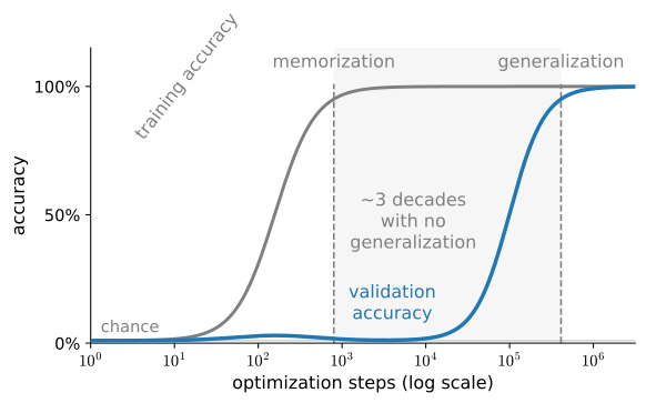
On small algorithmic tasks, a network first memorizes the training set, with test accuracy flat near chance.
Then, after orders of magnitude more steps at zero training loss, it suddenly generalizes, long after any early-stopping rule would have given up.
Same architecture, same data, same loss: only time spent training changes the outcome. Dynamics, not architecture alone, govern generalization.
Implicit bias
Networks have parameters, yet often behave like nonparametric models, whose complexity grows with the data.
As a randomly initialized MLP grows infinitely wide, it becomes equivalent to a kernel method for a fixed kernel:
the neural tangent kernel, a distance function the architecture induces.
Memorization and generalization can coexist: 1-nearest-neighbor memorizes everything, achieves zero training error, and still lands asymptotically within a factor of two of the optimal Bayes error (Cover & Hart, 1967).
Over-parametrized nets likewise interpolate, so the nonparametric intuition is often the more reliable one.
04
Regularization in practice
early stopping and classical penalties, reinterpreted
Practice
With label noise, networks fit the cleanly labeled examples first and only later interpolate the mislabeled ones.
Stop while the clean data is fit but the noise is not, and you can certify generalization (with high probability).
Patience criterion: monitor validation error each epoch; stop when it fails to improve by \epsilon for a few epochs. It also saves training time and money.
Matters most under label noise or intrinsic label variability. On clean, separable data it changes little.
Practice
Weight decay adds a norm penalty to the loss:
\ell_2\ (\text{ridge}):\ \lambda\lVert\mathbf{w}\rVert_2^2 \qquad \ell_1\ (\text{lasso}):\ \lambda\lVert\mathbf{w}\rVert_1.
But at typical strengths, \ell_2 is too weak to stop a network from interpolating the data.
So its benefit may come not from constraining capacity but from encoding a better inductive bias, much like the choice of distance in k-NN. Often it helps only together with early stopping. (Dropout is the next such tool.)
Wrap-up
Why certain choices improve generalization remains a massive open question. Try the surprises yourself: exercise 6 reproduces epoch-wise double descent; exercise 7, grokking on modular addition. Next (the dropout section): dropout, regularization by structured noise.