Regularizing with dropout Randomly mask hidden activations during training and evaluate the full network at test time.
A network with room to memorize
Motivation
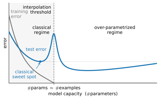
Modern nets are overparameterized: more weights than training points. Past the interpolation threshold, plain gradient descent can drive training error to zero by memorizing.
We want to retain capacity while discouraging the model from fitting peculiarities of the training set.
Test error past the interpolation threshold: capacity alone does not ensure generalization.
Dropout randomly masks hidden activations
The idea
Srivastava, Hinton et al. (2014) gave a simple definition:
Each training step, set each hidden unit to zero independently with probabilityp, then rescale the survivors by1/(1-p). At test time, turn it off.
Although dropout removes part of the network on each training step, it can improve generalization and is used in many Transformer configurations.
01
Why It Works
three views: a thinned net, an ensemble, broken co-adaptation
View 1: each step trains a thinned subnetwork
Why It Works
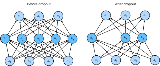
Zeroing units removes them from this step’s forward and backward pass. What is left is a thinned subnetwork; the next step samples a different one.
Here h_2 and h_5 are dropped, so the output cannot depend on them, and no single unit can dominate.
A single dropout draw: two of five hidden units zeroed, leaving a thinned network.
View 2: an exponentially large ensemble
Why It Works
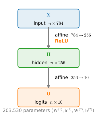
A net with n hidden units has 2^n possible masks, so 2^n thinned subnetworks, all sharing one set of weights. Today’s model has two 256-unit layers: 2^{512} \approx 10^{154} subnetworks.
Train: sample one mask per step; the update nudges the shared weights to help that subnetwork.
Test: run the full net with dropout off, which serves as a computational surrogate for the masked subnetworks.
The ensemble view is historical motivation. In a nonlinear network, the full test-time pass is not generally the arithmetic or geometric mean of the masked networks. Only the activation-level expectation is exact.
View 3: noise breaks co-adaptation
Why It Works
Because no unit can count on any specific partner being present, each is pushed to learn a feature that is useful on its own:
Anti-co-adaptation: robust, redundant features instead of features that only work in specific combinations.
Smoothness: Bishop (1995) showed that input-noise injection is equivalent to a smoothness (Tikhonov) penalty on the learned function; dropout is the same idea moved inside the network.
Three lenses, one mechanism: structured noise during training.
The arithmetic: keep the expectation
Why It Works
Replace each activation h with the random variable
The factor 1/(1-p) is the unique constant that keeps \mathbb{E}[h'] = p\cdot 0 + (1-p)\dfrac{h}{1-p} = h.
Rescaling during training is inverted dropout, what every modern framework implements. The original 2014 formulation instead multiplied the weights by 1-p at test time, equivalent in expectation, but inverting moves all bookkeeping into training, which is exactly why a Dropout layer can be a no-op in eval.
02
From Scratch
mask, rescale, and drop in the forward pass
A dropout layer in three lines
From Scratch
Sample a Bernoulli keep-mask from a uniform draw, multiply, then rescale the survivors by 1/(1-p) to restore the expectation:
p = 0.5 → about half the entries zero, survivors doubled (1/(1-0.5)=2).
p = 1 → everything dropped (degenerate).
Where dropout goes in an MLP
From Scratch
Apply it to each hidden layer’s output, after the activation:
Linear → ReLU → Dropout → Linear → ReLU → Dropout → Linear
Convention: a smaller rate near the input (low-level features must stay reliable), larger deeper in. Active in training only.
Dropout sits on the hidden activations of the MLP.
The model: two hidden layers, dropout gated on training
From Scratch
dropout_layer slots into forward right after each hidden activation, guarded by the training flag so evaluation always runs the full, unmasked network:
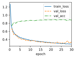
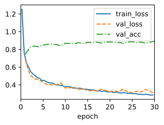
Two 256-unit hidden layers, dropout 0.2 after the first and 0.5 after the second (the gentler-near-the-input convention in action), on Fashion-MNIST:
The displayed train and validation curves track closely across 30 epochs. A causal claim about dropout would require a seed-matched no-dropout run under the same training settings.
03
Concise
one stock layer, train/eval handled for you
The framework Dropout layer
Concise
nn.Dropout(p) is a stock layer that also knows the train vs. eval switch: in eval mode it becomes a no-op, with no rescaling needed.
With the same hyperparameters, the layer performs the masking and rescaling internally:
model = DropoutMLP(**hparams)trainer.fit(model, data)
Dropout today
Current practice
Dropout usage depends on the architecture, dataset size, and training scale.
CNNs often combine data augmentation, normalization, weight decay, and stochastic depth, using dropout selectively.
Transformers may apply dropout to embeddings, attention and MLP blocks, or output heads. Rates from 0.0–0.1 are common, while some large-scale configurations use a rate of zero.
In the configuration where dropout is placed before batch norm, masking can distort the running variance and create an evaluation-time mismatch (Li et al., 2019).
Dropout is a low-cost regularizer that can be combined with weight decay and data augmentation. It also motivated a broader family of stochastic regularization methods.
Summary
Wrap-up
Dropout zeros each hidden unit with probability p during training, then rescales survivors by 1/(1-p).
The rescaling keeps \mathbb{E}[h']=h (inverted dropout), so test-time code is unchanged.
Off at test time: the full network runs, unmasked.
Place it after the activation, before the next linear layer; gentler near the input (0.2, then 0.5 here).
Proposed views include a thinned subnetwork each step, historical ensemble motivation, and reduced co-adaptation; only the masking expectation is exact.
nn.Dropout(p) does it all and respects train/eval.
Exercise 5 keeps dropout on at test time: average 20 passes, and you get uncertainty estimates (MC dropout). Next, the Kaggle house-prices section applies the methods from this chapter, deployed on a Kaggle competition.