import numpy as onp
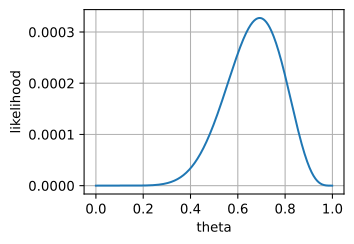
theta = onp.arange(0, 1, 0.001)
p = theta**9 * (1 - theta)**4.

d2l.plot(theta, p, 'theta', 'likelihood')Maximum Likelihood
Dive into Deep Learning · §27.3
The principle that turns a probabilistic model into a trainable loss
maximum likelihood.
Why maximum likelihood?
Motivation
Pick the parameters that maximize the observed-data probability mass or density. Many standard supervised losses are negative log-likelihoods for a chosen observation model.
- An operational recipe (the NLL you minimize).
- A geometry (empirical KL for discrete data; population KL under the continuous-data conditions stated below).
- An efficiency result for regular, identifiable models.
01
The principle and the coin
from Bayes to the likelihood, and the log trick
Likelihood and the flat prior
The principle
Start from the posterior and drop what does not depend on \boldsymbol\theta:
\hat{\boldsymbol\theta} = \operatorname*{argmax}_{\boldsymbol\theta} \frac{P(X\mid\boldsymbol\theta)\,P(\boldsymbol\theta)}{P(X)}.
P(X) is constant; a flat prior drops P(\boldsymbol\theta) too.
\hat{\boldsymbol\theta}_{\text{MLE}} = \operatorname*{argmax}_{\boldsymbol\theta} P(X\mid\boldsymbol\theta): maximum likelihood is MAP with a flat prior.
The coin: a likelihood surface
The coin
For 9 heads and 4 tails, P(X\mid\theta)=\theta^9(1-\theta)^4. Setting the derivative to zero gives
\hat\theta = \frac{n_H}{n_H+n_T} = \frac{9}{13}.
The MLE of a coin’s bias is always the observed frequency.
The negative log-likelihood
The log trick
A product of probabilities underflows; the log turns it into a sum and the gradient into a per-example sum (so SGD works):
\ell(\boldsymbol\theta) = -\sum_{i=1}^n \log p(x_i\mid\boldsymbol\theta).
(array(0.9713101), 0.9713101437890875)02
Maximum likelihood is minimizing a loss
cross-entropy, mean squared error, and the KL projection
Discrete MLE = minimum cross-entropy
Equivalences
Pool the data by outcome, \hat p_{\text{data}}(x)=n_x/n. Then
\tfrac1n\,\ell(\boldsymbol\theta) = \operatorname{CE}\bigl(\hat p_{\text{data}}, p_{\boldsymbol\theta}\bigr) = -\sum_x \hat p_{\text{data}}(x)\log p_{\boldsymbol\theta}(x).
Proof. Group identical observations and divide by n>0, an argmin-preserving rescaling. \blacksquare So maximizing likelihood is minimizing cross-entropy to the data.
Discrete empirical KL projection
KL geometry
For discrete outcomes, cross-entropy splits into a fixed empirical entropy plus a gap:
\operatorname{CE}(\hat p_{\text{data}}, p_{\boldsymbol\theta}) = H(\hat p_{\text{data}}) + D_{\mathrm{KL}}\bigl(\hat p_{\text{data}}\,\|\,p_{\boldsymbol\theta}\bigr).
Training changes only the KL term. For continuous observations, the analogous KL interpretation is a population statement under common-measure and integrability conditions, not a KL from the atomic empirical measure.
Gaussian NLL = mean squared error
Loss ↔︎ noise
With a fixed-variance Gaussian noise model,
-\log\!\prod_i \mathcal N(y_i;\hat y_i,\sigma^2) = \frac{1}{2\sigma^2}\sum_i (y_i-\hat y_i)^2 + \tfrac{n}{2}\log(2\pi\sigma^2).
The second term is \boldsymbol\theta-free, so the argmin is least squares.
Choosing a loss is choosing a noise model: Gaussian → MSE, Bernoulli → BCE, categorical → CE, Laplace → MAE.
From probabilities to densities
Continuous data
For a continuous x_i, the probability of the \epsilon-window is \approx \epsilon\,p(x_i\mid\boldsymbol\theta), contributing a constant -n\log\epsilon to the NLL.
That constant is \boldsymbol\theta-free and drops; the same NLL machine runs unchanged on densities.
03
Why maximum likelihood works
consistency, Fisher information, the Cramér–Rao floor
Consistency under assumptions
Estimator theory
For i.i.d. data from a well-specified model, the population objective is minimized at the truth. If that optimum is unique and identifiable and the empirical objective converges uniformly, then \hat{\boldsymbol\theta}\xrightarrow{P}\theta^\star.
Neural-network parameters are generally non-identifiable: several weight vectors may express the same function. A consistency result must therefore specify whether its target is a parameter-equivalence class, a function, or a distribution.
Asymptotic normality, watched
Estimator theory
Consistency says where \hat{\boldsymbol\theta} lands; the sharper statement is how tightly: \sqrt{n}\,(\hat{\boldsymbol\theta}-\boldsymbol\theta^\star) \xrightarrow{d} \mathcal N(\mathbf 0,\, I(\boldsymbol\theta^\star)^{-1}). This requires an interior true parameter, sufficient smoothness and moments, fixed support, and finite nonsingular Fisher information. Twenty thousand coin datasets (n=400, \theta^\star=0.7), rescaled:
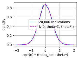
The histogram lands on the particular Gaussian the theorem names, \mathcal N(0,\,0.21): center, width, and height. Halving the error costs four times the data.
Fisher information
Curvature = information
The score is s = \nabla_{\boldsymbol\theta}\log p; the Fisher information is its variance, equivalently the expected NLL curvature:
I(\boldsymbol\theta) = \operatorname{Var}[s] = -\,\mathbb E\bigl[\nabla^2\log p\bigr].
A sharper NLL bowl pins the estimate down tighter. For the coin, I(\theta)=1/(\theta(1-\theta)).
Cramér–Rao: the efficiency floor
Curvature = information
No unbiased estimator beats the inverse Fisher information, and the MLE attains it asymptotically:
\operatorname{Var}(\tilde\theta) \ge \frac{1}{n\,I(\theta)}, \qquad \sqrt{n}\,(\hat{\boldsymbol\theta}-\theta^\star) \xrightarrow{d} \mathcal N\bigl(\mathbf 0, I(\theta^\star)^{-1}\bigr).
A simulation lands right on the Cramér–Rao floor:
(0.00103853717775, 0.00105)04
MAP: priors as regularizers
weight decay, sparsity, pseudo-counts
A Gaussian prior is weight decay
MAP
Keep the prior; its negative log is a penalty on the NLL. A \mathcal N(\mathbf 0,\tau^2 I) prior contributes \tfrac{1}{2\tau^2}\|\boldsymbol\theta\|_2^2:
\hat{\boldsymbol\theta}_{\text{MAP}} = \operatorname*{argmin}_{\boldsymbol\theta}\Bigl[ -\textstyle\sum_i\log p(x_i\mid\boldsymbol\theta) + \tfrac{1}{2\tau^2}\|\boldsymbol\theta\|_2^2\Bigr].
With Gaussian data this is ridge regression, \lambda=\sigma^2/\tau^2; a Laplace prior gives \ell_1 / sparsity.
A Beta prior on the coin
MAP
A \text{Beta}(a,b) prior shifts the optimum by pseudo-counts:
\hat\theta_{\text{MAP}} = \frac{n_H + a - 1}{n + a + b - 2}.
\text{Beta}(1,1) recovers the MLE; as n grows the prior washes out.
MAP returns the posterior mode, a point estimate, not the full posterior; the posterior mean differs (Laplace’s rule).
05
Latent variables, the ELBO, and EM
Jensen’s bound and coordinate ascent
Why latents break the recipe
Latent variables
With latents z the likelihood is a marginal, p(x;\boldsymbol\theta)=\sum_z p(x,z;\boldsymbol\theta), a sum inside the log (mixtures, VAEs, diffusion) that couples all parameters.
The complete-data problem (if we knew z) would be easy; the plan is to use that easy problem as a stepping stone.
The evidence lower bound
ELBO
For any q(z), Jensen gives a lower bound whose gap is a KL:
\log p(x;\boldsymbol\theta) = \underbrace{\mathbb E_q[\log p(x,z;\boldsymbol\theta)] + H(q)}_{\mathcal L(q,\boldsymbol\theta)} + D_{\mathrm{KL}}\bigl(q\,\|\,p(z\mid x)\bigr).
The bound is tight exactly when q is the posterior p(z\mid x).
EM: coordinate ascent on the ELBO
EM
E-step q_i = p(z\mid x_i;\boldsymbol\theta^{(t)}) closes the gap; M-step maximizes the expected complete-data log-likelihood. Exact steps never decrease the observed-data likelihood:
step  0, log-likelihood -1289.53
step  5, log-likelihood -845.69
step 10, log-likelihood -845.45
step 15, log-likelihood -845.45
step 20, log-likelihood -845.45
step 25, log-likelihood -845.45
step 30, log-likelihood -845.45
pi = [0.594 0.406], mu = [-2.055  1.494], sigma = [0.715 0.625]
This is a monotonicity guarantee, not a global-optimum guarantee. Approximate or stochastic updates require their own analysis.
Recap
Wrap-up
- MLE = maximize \sum_i\log p(x_i\mid\boldsymbol\theta) = minimize the NLL.
- For discrete data, average NLL is empirical cross-entropy and a KL projection; continuous-data KL statements are population statements. Consistency and efficiency require the assumptions stated above.
- Many common supervised losses are NLLs of an observation model; MSE is the fixed-variance Gaussian case.
- Priors become regularizers: Gaussian → weight decay, Laplace → sparsity, Beta → pseudo-counts.
- Latents: the ELBO lower-bounds the evidence with a KL gap; EM closes it then climbs.
- One principle threads classifiers, regressors, and generative models.