Constrained Optimization and Duality

Dive into Deep Learning · §25.4

Reading a constrained problem and its dual
Lagrange multipliers · KKT · projections · duality.

One idea, three guises

Motivation

At an unconstrained minimum the gradient vanishes. At a constrained minimum it need not, but there is no feasible descent direction: no move that both stays feasible and lowers f.

Equality constraints give Lagrange multipliers, \nabla f = -\nu\,\nabla g.
Inequality constraints give the KKT conditions.
Convex feasible sets make it an algorithm: projected gradient descent.

Every multiplier is a price: what relaxing its constraint is worth.

Lagrange multipliers

equality constraints and tangency

No feasible descent forces tangency

Lagrange

Where a level set of f crosses the constraint, \nabla f has a component along it, so sliding feasibly lowers f. Only where the curves are tangent does every feasible move stall, and tangency of the curves means their normals are parallel:

\nabla f(\mathbf{x}^\star) + \nu^\star\,\nabla g(\mathbf{x}^\star) = \mathbf{0}.

Valid wherever \nabla g(\mathbf{x}^\star) \neq \mathbf{0}, the constraint qualification.

The Lagrangian packages it

Lagrange

Parallel gradients and feasibility become joint stationarity of one function of more variables:

\mathcal{L}(\mathbf{x}, \nu) = f(\mathbf{x}) + \nu\, g(\mathbf{x}), \qquad \nabla_{\mathbf{x}}\mathcal{L} = \mathbf{0},\;\; \partial_\nu \mathcal{L} = g = 0.

Closest point on a hyperplane \mathbf{a}^\top\mathbf{x} = b: stationarity forces \mathbf{x} along the normal \mathbf{a}, giving \mathbf{x}^\star = \tfrac{b}{\|\mathbf{a}\|^2}\,\mathbf{a}.

Already a shadow price: \partial p^\star/\partial b = -\nu^\star. The multiplier tracks how the optimum moves when the constraint moves.

The KKT conditions

inequalities and the active set

Active, inactive, and a one-way push

KKT

With g_i(\mathbf{x}) \le 0, each constraint is inactive (g_i < 0, locally irrelevant) or active (g_i = 0, pushing back like an equality). At the optimum -\nabla f is a nonnegative combination of the active outward normals, in their cone.

An inequality multiplier carries a sign: \lambda_i \ge 0. It can push one way only, into the feasible side.

The four KKT conditions

KKT

Stationarity: \nabla f + \sum_i \lambda_i \nabla g_i + \sum_j \nu_j \nabla h_j = \mathbf{0}

Primal feas.: g_i \le 0,\;\; h_j = 0

Dual feas.: \lambda_i \ge 0

Comp. slackness: \lambda_i\, g_i = 0

Complementary slackness finds the active set: for each i, either g_i = 0 (active, \lambda_i free) or \lambda_i = 0 (slack, priced at zero). The pattern of zero multipliers tells you which constraints shaped the answer.

Convex f, g_i and affine h_j: a KKT point is a global minimum, by a three-line convexity argument. KKT is the answer.

Projections

making constraints an algorithm

Project, then it is an algorithm

Projections

\Pi_C(\mathbf{y}) is the nearest feasible point. On a convex set it is nonexpansive (\|\Pi_C\mathbf{x} - \Pi_C\mathbf{y}\| \le \|\mathbf{x} - \mathbf{y}\|), so appending it keeps gradient descent’s guarantees:

\mathbf{x}_{t+1} = \Pi_C\!\left(\mathbf{x}_t - \eta\,\nabla f(\mathbf{x}_t)\right).

Its fixed points are exactly the constrained optima, equivalent to KKT.

You have run PGD in disguise: gradient clipping projects onto a ball; non-negativity is a projection onto the orthant; max-norm weight caps project each row.

Simplex projection = sort, shift, clip

Projections

Projecting onto \{\mathbf{x} \ge 0,\, \sum_i x_i = 1\} is a QP the KKT conditions solve in closed form up to one threshold \tau:

x_i^\star = \max(y_i - \tau,\, 0), \qquad \textstyle\sum_i \max(y_i - \tau,\, 0) = 1.

Soft-threshold then renormalize. This is sparsemax: genuinely sparse attention weights, with complementary slackness choosing the zeros.

x* = [0.0676 0.     0.5823 0.0467 0.     0.3034]  sum = 1.000000
KKT residuals: stationarity 5.6e-17 | comp. slack 0.0e+00 | dual feas. 0.0e+00
f(x*) = 0.158962 <= best random feasible 0.162139

Two coordinates came back exactly zero, the active sign constraints; every KKT residual sits at machine precision.

Duality

bounds for free, and shadow prices

The dual function: bounds for free

Duality

Minimize the Lagrangian over \mathbf{x} to promote the multipliers to variables:

g(\boldsymbol{\lambda}, \boldsymbol{\nu}) = \inf_{\mathbf{x}}\, \mathcal{L}(\mathbf{x}, \boldsymbol{\lambda}, \boldsymbol{\nu}).

Always concave (an infimum of affine functions), even for a non-convex primal.
Weak duality: d^\star \le p^\star always. Every dual point certifies a lower bound.

Strong duality and shadow prices

Duality

Slater: convex problem + one strictly feasible point \Rightarrow d^\star = p^\star, the gap closes.

The dual is always convex, often the easier problem, and at strong duality solving it solves the primal.

Shadow price:

\lambda_i^\star = -\frac{\partial p^\star}{\partial u_i}.

Relax constraint i by a unit and the optimum improves by \lambda_i^\star.

Slack constraints cost nothing; only binding ones command a price.

Strong duality is a saddle point

Duality

The primal is \inf_{\mathbf{x}} \sup_{\boldsymbol{\lambda} \succeq 0} \mathcal{L} in disguise (a violated constraint lets its multiplier blow the sup to +\infty); the dual plays the same game in the other order. Weak duality is the universal \sup\inf \le \inf\sup (playing second is an advantage), and strong duality says the order of play does not matter:

\mathcal{L}(\mathbf{x}^\star, \boldsymbol{\lambda}) \;\le\; \mathcal{L}(\mathbf{x}^\star, \boldsymbol{\lambda}^\star) \;\le\; \mathcal{L}(\mathbf{x}, \boldsymbol{\lambda}^\star).

This is the shape of minimax training: GANs and adversarial training are \min_{\boldsymbol{\theta}}\max_{\boldsymbol{\phi}} problems, and “does a saddle point exist?” is exactly “is there a duality gap?”. Primal–dual methods descend in \mathbf{x}, ascend in \boldsymbol{\lambda}, and converge to the saddle.

Weight decay is a norm constraint

Duality at work

The two faces of \ell_2 regularization are one Lagrangian apart:

\underbrace{\min_{\mathbf{w}}\, L(\mathbf{w}) + \lambda\|\mathbf{w}\|^2}_{\text{penalty}} \;\Longleftrightarrow\; \underbrace{\min_{\mathbf{w}}\, L(\mathbf{w}) \;\text{s.t.}\; \|\mathbf{w}\|^2 \le r^2}_{\text{constraint}}

Same stationarity equation, \lambda playing the multiplier: \lambda = -\partial p^\star/\partial(r^2) prices the weight budget. Verified on ridge regression, where the theorem is exact:

 lambda    r = |w_pen|   |w_con - w_pen|   recovered multiplier
   0.10       0.4460         9.23e-17             0.1000
   1.00       0.4235         9.64e-17             1.0000
  10.00       0.2840         5.55e-17            10.0000

One number, three readings: weight decay (the weight-decay section), a norm budget’s shadow price, and a Gaussian prior (the maximum-likelihood section).

Worked: the SVM dual

Duality at work

Eliminate (\mathbf{w}, b) from the max-margin Lagrangian and the dual is a concave QP over the orthant, made for projected gradient ascent:

\max_{\boldsymbol{\alpha} \succeq 0}\;\; \mathbf{1}^\top \boldsymbol{\alpha} - \tfrac12 \boldsymbol{\alpha}^\top Q\, \boldsymbol{\alpha}, \qquad \boldsymbol{\alpha} \leftarrow \max(\mathbf{0},\, \boldsymbol{\alpha} + \eta\,(\mathbf{1} - Q\boldsymbol{\alpha})).

alpha* = [0.1309 0.0732 0.     0.     0.     0.2442 0.     0.3885]
w* = [0.5714 0.5714]  b* = -0.4286  separates data: True
margins y_i (w^T x_i + b) = [1.     1.     2.1429 2.1429 1.2857 1.     2.4286 1.    ]
KKT: comp. slack 3.0e-16 | worst primal feas. 7.8e-16
primal = 0.418367, dual = 0.418367, gap = 4.4e-16

The four nonzero \alpha_i are exactly the points at margin 1, the support vectors. Primal meets dual at 10^{-16}: strong duality, observed.

Worked: water-filling

Duality at work

Allocate power P across noisy channels. KKT pours until every wet channel reaches a common level w; complementary slackness keeps high-noise channels dry:

p_i^\star = \max(w - n_i,\, 0), \qquad \textstyle\sum_i \max(w - n_i, 0) = P.

The multiplier \mu = 1/w is literally the marginal value of power; the run below confirms it by finite differences, 0.697674 both ways.

A duality gap you can see

Duality at work

Weak duality never fails; strong duality can. Minimize the concave f_0 = -x^2 on [0,1] s.t. x \le \tfrac12:

p^\star = -\tfrac14, \qquad d^\star = -\tfrac12.

A strictly feasible point exists, yet the gap is real: Slater certifies strong duality only for convex problems.

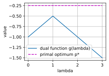
p* = -0.2500,  d* = -0.5000 at lambda = 1.00,  gap = 0.2500
weak duality g(lambda) <= p* everywhere: True

Recap

Wrap-up

A constrained optimum has no feasible descent direction, made precise by Lagrange and KKT; complementary slackness finds the active set.
Projections onto convex sets are nonexpansive; projected GD is gradient descent plus a snap back to feasibility.

The dual is always concave and always a lower bound; Slater closes the gap; multipliers are shadow prices.
SVM dual and water-filling are duality you can run; non-convexity leaves a gap you can see.

Many sub-problems of deep learning, projections, clipped updates, last-layer fits, live inside this convex toolkit.