import numpy as onp
def angle(v, w):
    return onp.arccos(v.dot(w) / (onp.linalg.norm(v) * onp.linalg.norm(w)))

angle(onp.array([0, 1, 2]), onp.array([2, 3, 4]))Geometric Interpretation of Linear Algebra
Motivation
A vector is a list of numbers with a useful geometric interpretation.
- A vector is a point, or equally an arrow (a direction).
- The dot product measures alignment, giving angles and similarity.
- A hyperplane is the decision boundary of every linear classifier.
- A matrix is a map that skews, rotates, and scales space.
These pictures are the foundation for the eigendecomposition and the SVD in the sections that follow.
Two readings of a vector
Vectors
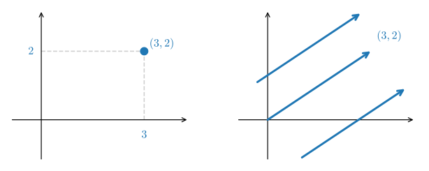
The same array denotes a point (its coordinates) or a direction (an arrow that may start anywhere). Deep learning often uses the direction view.
Reading a vector as a direction makes addition visual: follow one arrow, then the next, tip to tail.
Dot products and the angle
Vectors
Why is the dot product tied to the angle? The two vectors span a plane, so measure \|\mathbf{v}-\mathbf{w}\|^2 two ways and equate.
Algebra gives \|\mathbf{v}\|^2 - 2\,\mathbf{v}\cdot\mathbf{w} + \|\mathbf{w}\|^2; the law of cosines gives \|\mathbf{v}\|^2 + \|\mathbf{w}\|^2 - 2\,\|\mathbf{v}\|\,\|\mathbf{w}\|\cos\theta.
Cancel the common terms: \;\mathbf{v}\cdot\mathbf{w} = \|\mathbf{v}\|\,\|\mathbf{w}\|\cos\theta, so \theta=\arccos\!\big(\mathbf{v}\cdot\mathbf{w}/\|\mathbf{v}\|\,\|\mathbf{w}\|\big).
0.4189900840328574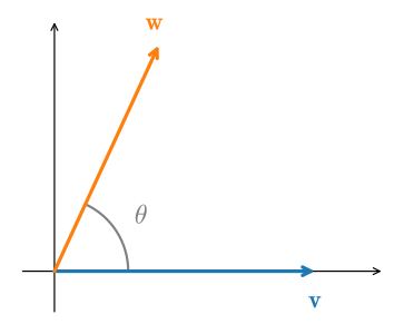
Projection and orthogonality
Vectors
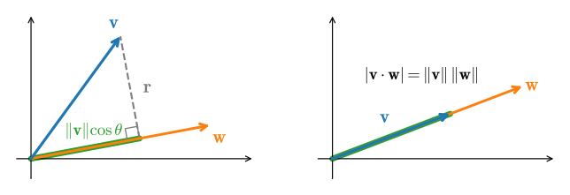
How much of \mathbf{v} points along \mathbf{w}? Drop \mathbf{v} onto the line through \mathbf{w}:
\operatorname{proj}_{\mathbf{w}}\mathbf{v} = \frac{\mathbf{v}\cdot\mathbf{w}}{\mathbf{w}\cdot\mathbf{w}}\,\mathbf{w}.
The residual \mathbf{r} is at a right angle to the projection direction, so Cauchy–Schwarz states that a leg is no longer than the hypotenuse. Two vectors are orthogonal when \mathbf{v}\cdot\mathbf{w} = 0.
This is least squares in one dimension (the best fit leaves an orthogonal residual); the SVD scales the same idea to any matrix.
Span, basis, dimension
Vectors
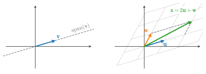
- Span: everything reachable by scaling and adding a set of vectors.
- Basis: an independent spanning set, so every vector gets unique coordinates.
- Dimension: the size of any basis.
Two subspaces ride on every matrix: the column space is what it can produce, the null space is what it sends to zero.
Random vectors are nearly orthogonal
High dimensions
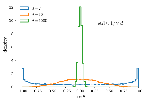
Drop two unrelated unit vectors into \mathbb{R}^d: what cosine do we expect?
For a random unit vector, \;\mathbb{E}[\cos\theta] = 0 and \operatorname{Var}(\cos\theta) = \tfrac{1}{d}.
Why: rotate so \mathbf{u}=\mathbf{e}_1, so \cos\theta=v_1. Symmetry \mathbf{v}\mapsto-\mathbf{v} kills the mean; \sum_i v_i^2=1 with all coordinates alike gives \mathbb{E}[v_1^2]=\tfrac{1}{d}.
Thus, the cosine concentrates at 0 with width 1/\sqrt{d}. Whether an observed cosine is meaningful depends on the dimension, candidate set, and learned representation.
A hyperplane as a decision boundary
Hyperplanes
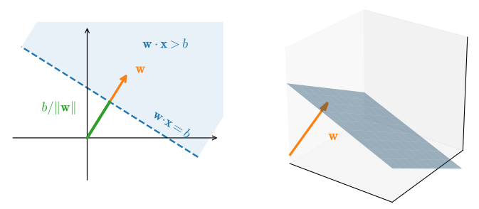
The set \{\mathbf{x} : \mathbf{w}\cdot\mathbf{x} = b\} is a plane with normal \mathbf{w}, sitting at distance b/\|\mathbf{w}\| from the origin. Sliding b translates it without rotating.
For any point, the signed distance (\mathbf{w}\cdot\mathbf{x} - b)/\|\mathbf{w}\| is positive on one side and negative on the other. That number is exactly a linear classifier’s margin.
Nearest-Centroid Linear Classifier
Hyperplanes
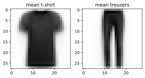
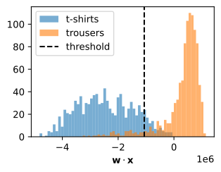
Take Fashion-MNIST t-shirts and trousers. Average each class: the means are blurry but recognizable. The line between them, \mathbf{w} = \overline{\mathbf{x}}_1 - \overline{\mathbf{x}}_0, is our normal.
Projection onto the Decision Normal
Hyperplanes
Reduce every image to one number, \mathbf{w}\cdot\mathbf{x}, its position along the normal. The two classes form two modes; the dashed threshold lies between them.
A learned classifier adjusts this boundary to reduce overlap; a deep network learns features that make the classes more readily separable.
Matrices as Linear Maps
Linear maps
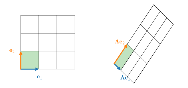
A matrix is fixed by where it sends the basis vectors, namely its columns. Every other vector follows as a weighted sum, so the entire grid is carried along: lines stay lines, the origin stays put, cells stay evenly spaced.
Matrices preserve linear combinations, though they may shear, rotate, reflect, project, or scale directions. Multiplying two matrices composes their maps.
Column Space and Null Space
Linear maps
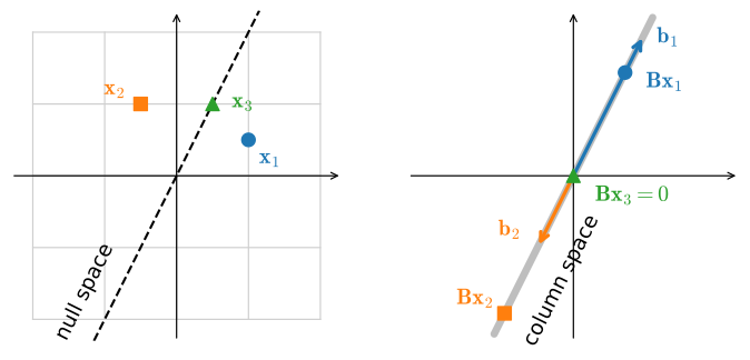
\mathbf{B} = \bigl[\begin{smallmatrix}2&-1\\4&-2\end{smallmatrix}\bigr] has dependent columns, \mathbf{b}_1 + 2\,\mathbf{b}_2 = \mathbf{0}. The whole plane lands on one line (the column space), and the direction (1,2)^\top is mapped to the origin (the null space). Once inputs collide, no inverse can tell them apart.
Rank–nullity. \operatorname{rank}\mathbf{A} + \dim\ker\mathbf{A} = n: of the n input dimensions, \dim\ker\mathbf{A} map to zero and \operatorname{rank}\mathbf{A} remain in the image. For \mathbf{B}: 1 + 1 = 2.
The determinant is signed area
Linear maps
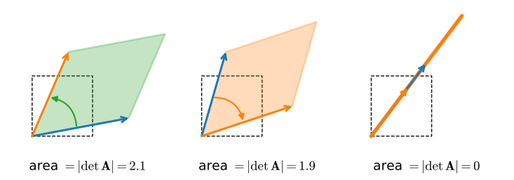
The unit square maps to a parallelogram; its signed area is \det\mathbf{A}. The sign records orientation, and a zero determinant means space was mapped to a lower dimension.
For our grid matrix, \det = 1\cdot3 - 2\cdot(-1) = 5:
import numpy as onp
onp.linalg.det(onp.array([[1, 2], [-1, 3]]))4.999999999999999Composed maps multiply their area scalings, \det(\mathbf{A}\mathbf{B})=\det\mathbf{A}\,\det\mathbf{B}. Two payoffs: \det\mathbf{Q}=\pm1 for orthogonal \mathbf{Q}, and (next section) \det\mathbf{A}=\prod_i\lambda_i, the per-axis stretches multiplied.