import numpy as onp
onp.linalg.eig(onp.array([[2, 1], [2, 3]]))Eigendecompositions
Dive into Deep Learning · §24.2
The directions a matrix only stretches
eigenvalues, the spectral theorem, and the spectral radius.
Eigenvalues and Iterated Linear Maps
Motivation
A matrix distorts space: it skews, rotates, rescales. Along special directions, the eigenvectors, the distortion is a pure stretch.
- An eigenbasis decouples the map into independent 1-D stretches.
- Powers \mathbf{A}^t then reduce to scalar powers \lambda^t; iterating \mathbf{A} aligns any input with the dominant eigenvector.
This drives PCA, covariance, the Hessian view of optimization, PageRank, and vanishing / exploding gradients.
01
Eigenvalues & eigenvectors
definition, geometry, the decomposition
The defining equation
The objects
A scalar \lambda and nonzero vector \mathbf{v} are an eigenpair of \mathbf{A} when
\mathbf{A}\mathbf{v} = \lambda\mathbf{v}.
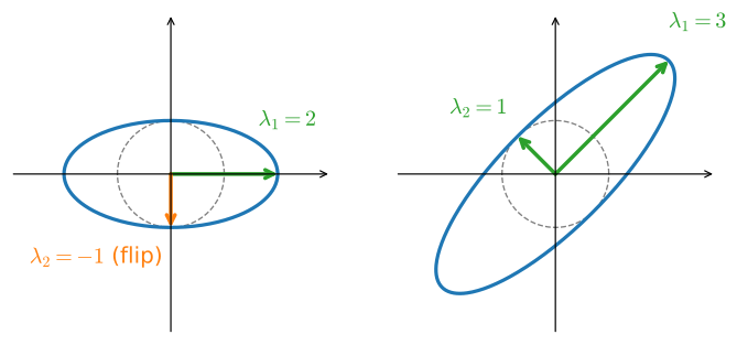
Take \mathbf{A}=\operatorname{diag}(2,-1): it doubles the x-axis and flips the y-axis. The axes themselves only change length, not direction, so [1,0]^\top and [0,1]^\top are eigenvectors with \lambda = 2 and \lambda = -1.
\lambda = 0 is allowed and signals a non-invertible matrix; only \mathbf{v}=\mathbf 0 is excluded.
The circle becomes an ellipse
The objects
For a symmetric matrix, the ellipse axes lie along the eigenvectors (green), with half-lengths |\lambda_i|:
Finding eigenvalues
The objects
\mathbf{A}\mathbf{v}=\lambda\mathbf{v} rearranges to (\mathbf{A}-\lambda\mathbf{I})\mathbf{v}=\mathbf 0. A nonzero solution exists only when that matrix is singular:
\det(\mathbf{A}-\lambda\mathbf{I}) = 0.
For \mathbf{A}=\bigl[\begin{smallmatrix}2&1\\2&3\end{smallmatrix}\bigr] this is (2-\lambda)(3-\lambda)-2=(4-\lambda)(1-\lambda), so \lambda=1,4 with eigenvectors [1,-1]^\top and [1,2]^\top (each defined up to scale).
Check it with eig
The objects
The library returns the same \lambda=1,4, with eigenvectors normalized to unit length (and an arbitrary sign), parallel to the ones we found by hand:
EigResult(eigenvalues=array([1., 4.]), eigenvectors=array([[-0.70710678, -0.4472136 ],
       [ 0.70710678, -0.89442719]]))
Real libraries never form the characteristic polynomial: they run the shifted QR algorithm on a Hessenberg reduction.
The eigendecomposition
The objects
Stack the eigenvectors as columns of \mathbf{W} and the eigenvalues on the diagonal of \boldsymbol{\Lambda}. Then \mathbf{A}\mathbf{W}=\mathbf{W}\boldsymbol{\Lambda}, and if \mathbf{W} is invertible (a diagonalizable matrix):
\mathbf{A} = \mathbf{W}\boldsymbol{\Lambda}\mathbf{W}^{-1}.
Powers reduce to scalar powers because the inner factors telescope:
\mathbf{A}^n = \mathbf{W}\boldsymbol{\Lambda}^n\mathbf{W}^{-1} \quad\Longrightarrow\quad \text{just raise each } \lambda_i \text{ to the } n.
Determinant & trace from the spectrum
The objects
\det is multiplicative and \operatorname{tr} is cyclic, so both ignore the change of basis in \mathbf{A}=\mathbf{W}\boldsymbol{\Lambda}\mathbf{W}^{-1}:
\det\mathbf{A} = \det\boldsymbol{\Lambda} = \prod_i \lambda_i, \qquad \operatorname{tr}\mathbf{A} = \operatorname{tr}\boldsymbol{\Lambda} = \sum_i \lambda_i.
Determinant is the product, trace the sum of the eigenvalues, and a diagonalizable matrix’s rank is the number of nonzero \lambda_i. Counted over \mathbb{C} with multiplicity, both identities hold for every square matrix (conjugate pairs keep them real).
When does an eigenbasis exist?
The objects
Diagonalizability is about counting eigenvectors. For each \lambda,
1 \le \underbrace{\dim(\text{eigenspace})}_{\text{geometric}} \le \underbrace{\text{root multiplicity}}_{\text{algebraic}},
and an eigenbasis exists iff these agree for every \lambda (n distinct eigenvalues guarantee it).
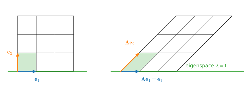
The shear \bigl[\begin{smallmatrix}1&1\\0&1\end{smallmatrix}\bigr] fails: \lambda=1 counts double, but the x-axis is the only line the map carries to itself. Defective: there is no second eigendirection to find.
Matrices Without an Eigenbasis
The objects
Over \mathbb{C}, every square matrix is similar to a block-diagonal matrix of Jordan blocks \mathbf{J}_k(\lambda): \lambda down the diagonal, 1s just above. Each block carries exactly one eigenvector, so geometric mult. = number of blocks, algebraic mult. = total size. The shear is \mathbf{J}_2(1).
\mathbf{J}_2(\lambda)^n = \lambda^n\mathbf{I} + n\lambda^{n-1}\mathbf{N}: the eigenvalue times a polynomial in n. For \lambda=0.99 the norm rises before it decays:
n =   1   ||J^n|| =    1.609   n * 0.99^(n-1) =    1.000
n =  50   ||J^n|| =   30.568   n * 0.99^(n-1) =   30.556
n = 100   ||J^n|| =   36.977   n * 0.99^(n-1) =   36.973
n = 200   ||J^n|| =   27.067   n * 0.99^(n-1) =   27.067
n = 800   ||J^n|| =    0.260   n * 0.99^(n-1) =    0.260
The full real inventory: stretch directions, Jordan blocks, rotation–scaling planes. Nothing else.
Complex eigenvalues are rotations
The objects
A planar rotation by \theta fixes no real direction, so it has no real eigenvector: its eigenvalues are the conjugate pair e^{\pm i\theta}, modulus 1 (length preserved), argument \pm\theta (the angle):
theta = np.pi / 6
R = np.array([[np.cos(theta), -np.sin(theta)],
              [np.sin(theta),  np.cos(theta)]])
print('eigenvalues of R:', np.round(np.linalg.eigvals(R), 4))
print('expected e^{+/- i*theta}:', np.round(np.exp([1j * theta, -1j * theta]), 4))
print('moduli (should be 1):', np.round(np.abs(np.linalg.eigvals(R)), 4))
eigenvalues of R: [0.866+0.5j 0.866-0.5j]
expected e^{+/- i*theta}: [0.866+0.5j 0.866-0.5j]
moduli (should be 1): [1. 1.]The dictionary: split the eigenvector of \lambda=a+ib as \mathbf{w}=\mathbf{u}+i\mathbf{v}. Then \textrm{span}\{\mathbf{u},\mathbf{v}\} is invariant, and with \mathbf{P}=[\mathbf{v}\;\;\mathbf{u}],
\mathbf{P}^{-1}\mathbf{A}\mathbf{P} = \left(\begin{smallmatrix} a & -b\\ b & \phantom{-}a \end{smallmatrix}\right) = r\left(\begin{smallmatrix} \cos\theta & -\sin\theta\\ \sin\theta & \phantom{-}\cos\theta \end{smallmatrix}\right).
Right to left: the block is multiplication by a+ib on \mathbb{R}^2\cong\mathbb{C}.
A real matrix’s complex eigenvalues come in pairs re^{\pm i\theta}: scale by r, rotate by \theta. That is why power iteration can spin instead of settling.
02
Symmetric matrices
the spectral theorem, positive definiteness, Rayleigh
The spectral theorem
Symmetry
Every real symmetric \mathbf{A}=\mathbf{A}^\top has a full orthonormal eigenbasis with real eigenvalues: \;\mathbf{A} = \mathbf{W}\boldsymbol{\Lambda}\mathbf{W}^\top, \;\mathbf{W}^\top\mathbf{W}=\mathbf{I}.
(i) eigenvalues are real. With the conjugate inner product, \lambda\|\mathbf{v}\|^2 = \mathbf{v}^*\!\mathbf{A}\mathbf{v} = (\mathbf{A}\mathbf{v})^*\mathbf{v} = \bar\lambda\|\mathbf{v}\|^2, so \lambda=\bar\lambda.
(ii) distinct eigenvalues give orthogonal eigenvectors. Sliding \mathbf{A}=\mathbf{A}^\top across the inner product, \lambda\langle\mathbf{u},\mathbf{v}\rangle = \langle\mathbf{A}\mathbf{u},\mathbf{v}\rangle = \langle\mathbf{u},\mathbf{A}\mathbf{v}\rangle = \mu\langle\mathbf{u},\mathbf{v}\rangle, so (\lambda-\mu)\langle\mathbf{u},\mathbf{v}\rangle=0.
(iii) an induction on the \mathbf{A}-invariant orthogonal complement \mathbf{w}_1^{\perp} fills out the basis. Geometrically \mathbf{A}=\mathbf{W}\boldsymbol{\Lambda}\mathbf{W}^\top is rotate (onto the axes), scale, rotate back, the ellipse picture, now guaranteed.
Applied to \mathbf{A}^\top\mathbf{A} (always symmetric, PSD), the same theorem builds the SVD for every matrix.
Eigenvalue Signs and Quadratic Forms
Symmetry
Rotating \mathbf{x} into the eigenbasis turns the quadratic form into a weighted sum of squares, \mathbf{x}^\top\mathbf{A}\mathbf{x}=\sum_i\lambda_i(\mathbf{w}_i^\top\mathbf{x})^2, so the eigenvalue signs are the surface shape:
Positive definiteness, in code
Symmetry
\mathbf{A}\succ0 iff every \lambda_i>0; \mathbf{A}\succeq0 iff every \lambda_i\ge0. A Gram matrix \mathbf{X}^\top\mathbf{X} is always PSD, and PD exactly when \mathbf{X} has full column rank:
X_full = np.array([[1., 0.], [1., 1.], [0., 1.], [2., 1.]])  # rank 2
X_dep = np.array([[1., 2.], [1., 2.], [0., 0.], [2., 4.]])   # col 2 = 2*col 1
for X, name in [(X_full, 'full column rank'), (X_dep, 'dependent columns')]:
    eigvals = np.linalg.eigvalsh(X.T @ X).round(4)
    eigvals[np.abs(eigvals) < 1e-9] = 0.0  # clean up tiny round-off / -0.0
    print(f'{name}: eigenvalues of X^T X = {eigvals}')
full column rank: eigenvalues of X^T X = [1.1459 7.8541]
dependent columns: eigenvalues of X^T X = [ 0. 30.]Full rank gives two positive eigenvalues (PD); dependent columns give a zero eigenvalue (PSD, not PD). This is the Hessian “is it a minimum?” test.
Eigenvalues as extreme stretches
Symmetry
The same weighted-average view bounds the Rayleigh quotient: it is a convex combination of the eigenvalues, so
\lambda_n \le \frac{\mathbf{x}^\top\mathbf{A}\mathbf{x}}{\mathbf{x}^\top\mathbf{x}} \le \lambda_1,
with the extremes hit at \mathbf{w}_1 and \mathbf{w}_n.
Sweeping a unit vector around the circle shows that the extrema of R match eigvalsh to the grid’s resolution and occur at the eigenvector angles:
sweep of R:  min = 1.381967, max = 3.618033
eigvalsh:    [1.381966 3.618034]
So \lambda_{\max} and \lambda_{\min} are the largest and smallest stretches. Their ratio \kappa=\lambda_{\max}/\lambda_{\min} is the condition number, what makes a steep-and-flat bowl slow to descend.
03
Locating & iterating
Gershgorin discs, power iteration, the spectral radius
Gershgorin discs
Dynamics
Bound the spectrum without computing it: every eigenvalue lies in the union of discs centered at a_{ii} with radius the off-diagonal row sum r_i=\sum_{j\neq i}|a_{ij}|.
Gershgorin: the bound is tight enough to use
Dynamics
For the symmetric matrix above, the four discs give the ranges [0.7,1.3], [2.4,3.6], [4.2,5.8], [8.1,9.9], and the true eigenvalues land inside each:
array([9.08033648, 0.99228545, 4.95394089, 2.97343718])Strict diagonal dominance with positive diagonal keeps 0 out of every disc, a no-computation proof of invertibility.
Power iteration
Dynamics
Why does iterating \mathbf{A} pick out one direction? Expand \mathbf{v}_0 in the eigenbasis and apply \mathbf{A} k times:
\mathbf{A}^k\mathbf{v}_0 = \lambda_1^k\Bigl(c_1\mathbf{w}_1 + \sum_{i\ge2} c_i\bigl(\tfrac{\lambda_i}{\lambda_1}\bigr)^{k}\mathbf{w}_i\Bigr).
Every ratio |\lambda_i/\lambda_1|<1, so the tail decays: the iterate aligns with \mathbf{w}_1 and the norm grows like |\lambda_1|^k.
Convergence of Power Iteration
Dynamics
The direction gap closes at rate |\lambda_2/\lambda_1|; the norm ratio settles onto \lambda_1 even faster:
Numerical Accuracy of Power Iteration
Dynamics
On a random 5\times5 matrix, the stabilized norm ratio matches \max_i|\lambda_i| to ten decimal places:
import numpy as onp
onp.random.seed(8675309)
A = onp.random.randn(5, 5)
v = onp.random.randn(5, 1)
for _ in range(200):
    Av = A @ v
    ratio = onp.linalg.norm(Av) / onp.linalg.norm(v)
    v = Av / onp.linalg.norm(Av)
rho = max(abs(onp.linalg.eigvals(A)))
print(f'stabilized norm ratio = {ratio:.10f}   max|eigenvalue| = {rho:.10f}')
stabilized norm ratio = 1.9744593215 max|eigenvalue| = 1.9744593215Large-Scale Applications of Power Iteration
Dynamics
PageRank is a dominant eigenvector. The fraction of time a random surfer spends on each page is the stationary \boldsymbol\pi with \mathbf{P}\boldsymbol\pi = \boldsymbol\pi, computed by power iteration: forming \mathbf{P} at web scale is unthinkable, multiplying by it is cheap.
The real web has dangling pages and disconnected pockets, so PageRank iterates the damped matrix
\alpha\,\mathbf{P} + (1-\alpha)\,\tfrac1n\mathbf{1}\mathbf{1}^\top, \qquad \alpha \approx 0.85,
a surfer who teleports to a random page with probability 0.15.
Damping makes every entry positive, so Perron–Frobenius applies by construction, and it guarantees the gap |\lambda_2| \le \alpha, so power iteration converges fast.
Spectra of Random Matrices
Random matrices
Form the sample covariance of pure noise: n samples of d independent unit-variance coordinates, true covariance \mathbf{I}. Its eigenvalues do not sit near 1; they spread deterministically over the Marchenko–Pastur bulk
\bigl[\,(1-\sqrt\gamma)^2,\ (1+\sqrt\gamma)^2\,\bigr], \qquad \gamma = d/n,
which for d = n/4 already spans [0.25,\ 2.25], from noise alone.
The bulk is the null hypothesis of spectral data analysis: an eigenvalue inside it is indistinguishable from sampling noise; only eigenvalues that escape above the edge testify to structure. That is the principled answer to “how many PCA components should I keep?”
Spectral radius & deep networks
Applications
The single number governing iterated maps is the spectral radius \rho(\mathbf{A})=\max_i|\lambda_i|, the asymptotic growth factor measured above.
- Backprop-through-time multiplies per-step Jacobians: the gradient scales like \rho^{T}.
- \rho>1 explodes, \rho<1 vanishes: either kills long-range learning.
- For random weights the circular law gives \rho\!\sim\!\sqrt{n}, hence the 1/\sqrt{\text{fan-in}} initialization that keeps \rho\approx1.
Keep \rho\approx1: the principle behind orthogonal init, gradient clipping, and LSTM/GRU gating.
Eigenstructure governs repeated square maps
Wrap-up
- \mathbf{A}\mathbf{v}=\lambda\mathbf{v}: eigenvectors are stretched, not rotated; the circle becomes an ellipse.
- \mathbf{A}=\mathbf{W}\boldsymbol{\Lambda}\mathbf{W}^{-1} turns powers, \det, and \operatorname{tr} into scalar facts.
- Symmetric \Rightarrow orthonormal eigenbasis, real \lambda: the foundation of PCA and the SVD.
- The sign of \lambda decides positive definiteness; the spread decides conditioning.
- Gershgorin localizes \lambda cheaply; power iteration finds the dominant one, which is how PageRank is computed.
- The spectral radius \rho governs stability, from RNN gradients to weight initialization.
Keeping the largest eigenvalue modulus near 1 is what ties this section to deep-network training.