Brownian motion, Itô calculus, and the SDE a continuous-time model for diffusion forward processes.
Noise supplies a data-independent forward process
Motivation
No fixed map can forget every dataset: a data-independent bijection sends distinct laws to distinct endpoints, so no single deterministic flow carries everyp_{\text{data}} to the same \mathcal N(\mathbf 0, \sigma^2 I). Noise defines such a process without learned parameters:
d\mathbf X = \underbrace{\mathbf f(\mathbf X,t)\,dt}_{\text{drift}}
+ \underbrace{g(t)\,d\mathbf W}_{\text{diffusion}}.
(A learned flow sends one givenp_{\text{data}} there: that is exactly flow matching, the score-matching-diffusion-and-flow-matching section.)
01
Brownian motion
axioms, covariance, simulation
The Wiener process
Brownian motion
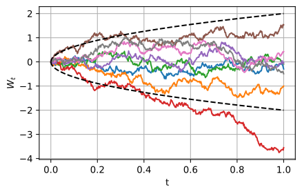
The \pm\sqrt{\Delta t} random walk has a non-degenerate limit W_t: W_0=0, independent increments, W_t-W_s\sim\mathcal N(0,t-s), continuous paths. Simulate with \Delta W = \sqrt{\Delta t}\,\xi, \xi\sim\mathcal N(0,1).
Covariance and non-differentiability
Brownian motion
\operatorname{Cov}(W_s,W_t) = \min(s,t).
Proof. Split W_t = W_s + (W_t-W_s); the cross term factorizes by independence and both factors are mean-zero. \blacksquare
The magnitude |\Delta W/\Delta t|=|\xi|/\sqrt{\Delta t} diverges in probability for a fresh increment. This scaling motivates, but does not prove, the theorem that Brownian paths are nowhere differentiable.
rng = np.random.default_rng(42)T, n, n_paths =1.0, 500, 20000dt = T / nt = np.linspace(0, T, n +1)dW = np.sqrt(dt) * rng.standard_normal((n_paths, n))W = np.concatenate([np.zeros((n_paths, 1)), np.cumsum(dW, axis=1)], axis=1)for s in [0.25, 0.5, 1.0]: k =round(s / dt)print(f'Var(W_t) at t={s:.2f}: {W[:, k].var():.4f} (theory: {s:.2f})')d2l.plot(t, [W[i] for i inrange(8)] + [2* np.sqrt(t), -2* np.sqrt(t)],'t', '$W_t$', fmts=['-'] *8+ ['k--', 'k--'], figsize=(5, 3))
Var(W_t) at t=0.25: 0.2486   (theory: 0.25)
Var(W_t) at t=0.50: 0.4950   (theory: 0.50)
Var(W_t) at t=1.00: 1.0014   (theory: 1.00)
02
Itô calculus
quadratic variation, the integral, the chain rule
Quadratic variation
Why ordinary calculus fails
For a smooth path \sum(\Delta x_i)^2\to 0. For Brownian motion it converges to the elapsed time:
\sum_i (\Delta W_i)^2 \longrightarrow t.
The Itô multiplication table
Why ordinary calculus fails
Proof.\mathbb E[\sum(\Delta W_i)^2]=\sum\Delta t_i=t exactly, and the variance is \sum 2\Delta t_i^2 \le 2\delta t\to 0. \blacksquare
(dW)^2 = dt, \qquad dW\,dt = 0, \qquad (dt)^2 = 0. A squared Brownian increment contributes at order dt.
Predictability makes the Itô integral non-anticipating
The integral
For a simple predictable process, choose G_i using information available at t_i and define \int_0^tG_s\,dW_s=\sum_iG_i\Delta W_i. Extend this definition to square-integrable predictable processes by the isometry. Since G_i\perp\Delta W_i,
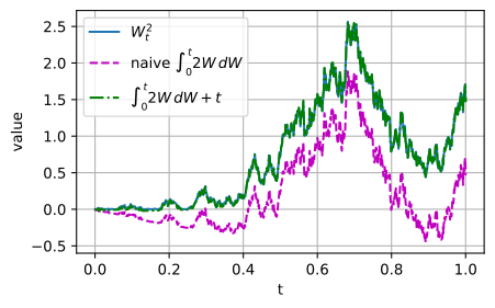
The \tfrac12 g^2\phi_{xx} term produces the diffusion term in the Fokker–Planck equation. Check \phi=x^2, X=W: d(W^2)=2W\,dW+dt, so \int_0^t W\,dW=\tfrac12(W_t^2-t):
rng = np.random.default_rng(3)T, n =1.0, 1000dt = T / nt = np.linspace(0, T, n +1)dW = np.sqrt(dt) * rng.standard_normal(n)W = np.concatenate([[0.0], np.cumsum(dW)])ito = np.concatenate([[0.0], np.cumsum(2* W[:-1] * dW)]) # left endpointprint(f'W_T^2 - int 2W dW = {W[-1]**2- ito[-1]:.4f} (Ito correction: T = {T})')print(f'max |gap_t - t| along the path = {np.abs(W**2- ito - t).max():.4f}')d2l.plot(t, [W**2, ito, ito + t], 't', 'value', legend=['$W_t^2$', 'naive $\\int_0^t 2W\\,dW$', '$\\int_0^t 2W\\,dW + t$'], figsize=(5, 3))
W_T^2 - int 2W dW = 1.0150   (Ito correction: T = 1.0)
max |gap_t - t| along the path = 0.0235
03
SDEs and Euler–Maruyama
the precise meaning, simulation, convergence
An SDE induces a distribution over paths
The objects
dX = f\,dt + g\,dW means X_t = X_0 + \int_0^t f\,ds + \int_0^t g\,dW_s. Here f is the mean velocity (\mathbb E[dX]=f\,dt) and g^2 the variance rate (\operatorname{Var}(dX)=g^2\,dt); a solution defines a distribution over paths, and g=0 recovers the ODE.
Euler–Maruyama: Euler plus a √Δt kick
Simulation
X_{n+1} = X_n + f(X_n,t_n)\,\Delta t + g(X_n,t_n)\sqrt{\Delta t}\,\xi_n.
The noise scales as \sqrt{\Delta t}, not \Delta t; g=0 is exactly forward Euler:
def euler_maruyama(f, g, x0, t, dW):"""Simulate dX = f dt + g dW on the grid t for a batch of paths.""" X = np.empty((len(x0), len(t))) X[:, 0] = x0for k inrange(len(t) -1): h = t[k +1] - t[k] X[:, k +1] = X[:, k] + f(X[:, k], t[k]) * h + g(X[:, k], t[k]) * dW[:, k]return Xt = np.linspace(0, 2.0, 201)X = euler_maruyama(lambda x, s: -x, lambda x, s: 0.0, np.ones(1), t, np.zeros((1, 200)))print('g = 0 recovers Euler on dx/dt = -x: 'f'max |X_t - e^(-t)| = {np.abs(X[0] - np.exp(-t)).max():.5f}')
g = 0 recovers Euler on dx/dt = -x: max |X_t - e^(-t)| = 0.00185
Strong and weak errors measure different quantities
Convergence
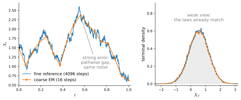
Strong error tracks one path against a fine reference driven by the same increments; weak error compares only the terminal laws. The coarse path visibly strays while the histograms already coincide. Endpoint-law sampling uses weak accuracy; path-coupled computations may require strong accuracy:
Euler–Maruyama has distinct strong and weak orders
Convergence
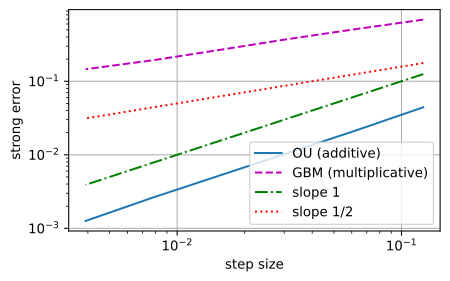
Under the standard Lipschitz and smoothness assumptions, strong order is \tfrac12 in general but improves to 1 for sufficiently regular additive noise: the omitted Milstein term carries \partial_x g, which vanishes. Weak order is 1 for sufficiently smooth coefficients and tests:
strong-order slopes: OU (additive) 1.02, GBM (multiplicative) 0.45
Measured slopes: additive OU \approx 1, multiplicative GBM \approx 0.5.
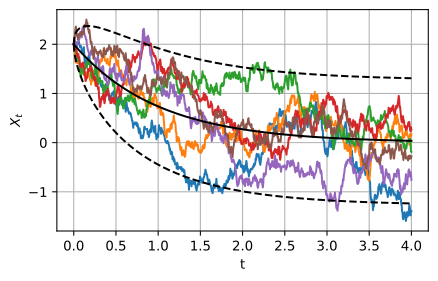
with relaxation time 1/\theta. The path cloud and its endpoint histogram confirm it:
t=0.5:  mean  1.2237 vs  1.2131,   std 0.4997 vs 0.5060
t=1.0:  mean  0.7336 vs  0.7358,   std 0.5912 vs 0.5918
t=2.0:  mean  0.2712 vs  0.2707,   std 0.6304 vs 0.6305
t=4.0:  mean  0.0406 vs  0.0366,   std 0.6399 vs 0.6363
fraction of paths inside the +-2 sigma band at t=4: 0.952   (Gaussian: 0.954)