lam_f = 50.0 # the test equation dx/dt = -50 x
T = 1.0
print('forward Euler is stable iff h < 2/lambda =', 2 / lam_f)
print(f'{"h":>8} {"|1-h*lam|":>10} {"forward x(T)":>14} {"backward x(T)":>14}')
for n in [10, 20, 26, 40, 100]:
h = T / n
fwd = (1 - h * lam_f) ** n # forward Euler after n steps
bwd = (1 + h * lam_f) ** (-n) # backward Euler after n steps
print(f'{h:8.3f} {abs(1 - h * lam_f):10.2f} {fwd:14.2e} {bwd:14.2e}')
print('exact x(T) = e^{-50} =', f'{np.exp(-lam_f * T):.2e}')
A_stiff = np.diag([-50.0, -1.0]) # one fast mode, one slow mode
x_stiff = euler(lambda x: A_stiff @ x, np.array([1.0, 1.0]), T, 20)
print('stiff system, forward Euler with h=0.05 '
'(the long-dead fast mode explodes):')
print('x(T) =', x_stiff.round(2))Ordinary Differential Equations and Numerical Solvers
Dive into Deep Learning · §29.1
A velocity field and the curves it generates
ODEs, numerical solvers, and Neural ODEs.
Exact dynamics and numerical updates are different objects
Motivation
A velocity field assigns a velocity at every point and time, and its solution is tangent to that field. Related constructions include:
- a residual update has the form of an Euler step,
- discrete backpropagation is a discrete adjoint,
- a continuous flow’s log-density change is a trace integral.
01
Vector fields and well-posedness
the IVP, the flow map, Picard–Lindelöf
The initial-value problem
The objects
A velocity field \mathbf f and a start \mathbf x_0 define
\dot{\mathbf x}(t) = \mathbf f(\mathbf x(t),t), \qquad \mathbf x(0)=\mathbf x_0, \qquad \mathbf x(t) = \mathbf x_0 + \int_0^t \mathbf f(\mathbf x(s),s)\,ds.
Euler’s method is just the left-endpoint Riemann sum of that integral.
The flow map
The objects
Collect all solutions into the map \Phi_t(\mathbf x_0) = \mathbf x(t):
\Phi_0 = \mathrm{id}, \qquad \Phi_{t+s} = \Phi_t\circ\Phi_s, \qquad \Phi_t^{-1} = \Phi_{-t}.
This inverse exists when the solution exists uniquely in both time directions. It is a property of the exact flow, not of an arbitrary Euler step.
Existence and uniqueness
Well-posedness
If \mathbf f is continuous in t and L-Lipschitz in \mathbf x, the IVP has a unique solution.
Proof. The Picard operator (P\varphi)(t)=\mathbf x_0+\int_0^t\mathbf f(\varphi(s),s)\,ds is a contraction on a short interval (\delta < 1/L); Banach’s fixed point gives existence + uniqueness, then patch intervals to cover [0,T]. \blacksquare
When uniqueness fails
Counterexamples
Without the Lipschitz bound, the solution is not unique: \dot x=\sqrt{|x|} from x(0)=0 can wait any time c then leave as (t-c)^2/4:
Drop the growth bound and \dot x = x^2 blows up in finite time at t=1/x_0.
02
Linear ODEs and stability
the matrix exponential, eigenvalues, phase portraits
The matrix exponential
Linear systems
For \dot{\mathbf x}=A\mathbf x the solution is \mathbf x(t)=e^{At}\mathbf x_0, where
e^{At} = \sum_{k=0}^{\infty}\frac{(At)^k}{k!}, \qquad e^{At}=V e^{\Lambda t}V^{-1}\quad\text{if }A=V\Lambda V^{-1}.
The eigenbasis decouples the system into independent scalar modes e^{\lambda_i t}, exactly the eigendecomposition machinery of the linear algebra part at work.
Three ways to the same map
Linear systems
Power series, eigendecomposition, and the Euler limit (I+tA/n)^n all agree, and the norm decays exactly as the theory predicts:
eigenvalues of A: [-0.5+1.j -0.5-1.j]
|series - eigen formula| : 5.6e-17
|(I+tA/n)^n - eigen|     : 5.4e-08
||e^{At} x0|| = 0.735759  vs  e^{-t/2}||x0|| = 0.735759
Stability from eigenvalues
Linear systems
Each mode’s size is |e^{\lambda_i t}| = e^{(\operatorname{Re}\lambda_i)t}:
\operatorname{Re}\lambda < 0 → decay; \operatorname{Re}\lambda > 0 → growth; \operatorname{Im}\lambda \ne 0 → oscillation. Eigenvalues determine asymptotic stability of the linear system, although nonnormal systems can have substantial transient growth.
Phase portraits
Linear systems
The eigenvalue signature names the picture (node, saddle, spiral, center):
At a nonlinear fixed point the Jacobian \partial\mathbf f/\partial\mathbf x gives the same local classification when the fixed point is hyperbolic (Hartman–Grobman). Eigenvalues on the imaginary axis require a separate analysis.
03
Numerical solvers
Euler, Runge–Kutta, stiffness, and gradient descent
Forward Euler, order one
Solvers
\mathbf x_{n+1} = \mathbf x_n + h\,\mathbf f(\mathbf x_n,t_n).
Local error O(h^2) per step; unrolling N=T/h steps and summing a geometric series gives global error O(h), amplified by the stability factor e^{LT}. The general rule: local O(h^{p+1}) → global O(h^p).
Runge–Kutta: probe inside the step
Solvers
RK4 samples four slopes (k_1 at the start, two at the midpoint, one at the end) and Simpson-weights them \tfrac16(k_1+2k_2+2k_3+k_4): global order 4, so halving h cuts error by 16.
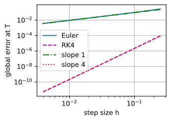
measured slope, Euler: 1.040
measured slope, RK4  : 4.022
The measured slopes are 1.0 (Euler) and 4.0 (RK4), matching theory.
Stiffness and implicit Euler
Solvers
On \dot x=-\lambda x, forward Euler is stable only for h < 2/\lambda; a rapidly decaying mode can therefore force a small step. Backward Euler is stable for every h (A-stable) at the cost of one solve per step, but a stable large step need not be accurate:
forward Euler is stable iff h < 2/lambda = 0.04
       h  |1-h*lam|   forward x(T)  backward x(T)
   0.100       4.00       1.05e+06       1.65e-08
   0.050       1.50       3.33e+03       1.31e-11
   0.038       0.92       1.25e-01       7.73e-13
   0.025       0.25       8.27e-25       8.18e-15
   0.010       0.50       7.89e-31       2.46e-18
exact x(T) = e^{-50} = 1.93e-22
stiff system, forward Euler with h=0.05 (the long-dead fast mode explodes):
x(T) = [3.32526e+03 3.60000e-01]
The stability picture
Solvers
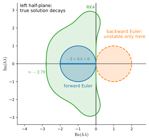
In the complex plane of z = h\lambda:
- forward Euler decays only inside the disc |1+z| < 1;
- RK4’s lobes stretch to \approx -2.79 on the real axis;
- backward Euler is stable everywhere but a disc, in particular on the entire left half-plane, which is A-stability.
Gradient descent is a solver
Training as dynamics
Gradient descent with learning rate \eta is forward Euler on the gradient flow \dot{\mathbf x} = -\nabla L(\mathbf x); near a minimum with Hessian H it linearizes onto the test equation:
\dot{\boldsymbol\delta} = -H\boldsymbol\delta \;\;\xrightarrow{\ \text{Euler},\ h=\eta\ }\;\; \boldsymbol\delta_{k+1} = (I-\eta H)\,\boldsymbol\delta_k \;\;\Longrightarrow\;\; \eta < \frac{2}{\lambda_{\max}(H)}.
A diverging learning rate is a solver instability; an ill-conditioned Hessian is a stiff gradient flow. Momentum is one derivative up: heavy-ball discretizes m\ddot{\mathbf x}+\gamma\dot{\mathbf x}=-\nabla L.
The gradient-descent stability threshold
Training as dynamics
On a quadratic with \lambda_{\max}=10 the predicted flip is \eta = 0.2: the sweep diverges already at \eta = 0.201, while the slow mode (\lambda=1) converges at every rate shown:
GD on this quadratic is stable iff eta < 2/lambda_max = 0.2
     eta  |1-eta*lam_max|  ||x|| after 100 GD steps
   0.050             0.50                  5.92e-03
   0.150             0.50                  8.75e-08
   0.190             0.90                  2.66e-05
   0.201             1.01                  2.70e+00
   0.210             1.10                  1.38e+04
   0.250             1.50                  4.07e+17
The unstable coordinate is the high-curvature mode, even while the low-curvature coordinate continues to contract.
04
Neural ODEs and continuous flows
residual updates, discrete and continuous adjoints, density traces
A residual update has Euler’s algebraic form
Architecture
\mathbf x_{l+1} = \mathbf x_l + \mathbf f_{\theta_l}(\mathbf x_l) is one Euler-shaped update at h=1. A continuous-depth limit additionally requires a consistent time-indexed field and shrinking steps:
The Neural ODE limit
Architecture
Shrink the step and the stack becomes \dot{\mathbf x}=\mathbf f_\theta(\mathbf x,t), \mathbf x(T)=\mathbf x_0+\int_0^T\mathbf f_\theta\,dt. A 1-hidden-layer net learns a circle→ellipse flow:
iter   0  loss 1.27961
iter 100  loss 0.00003
iter 200  loss 0.00001
iter 300  loss 0.00000
iter 400  loss 0.00000
mean endpoint error: 0.0013
The exact flow of a Lipschitz field is invertible over intervals with unique forward and backward solutions. Its finite numerical approximation need not be.
Continuous and discrete adjoints optimize different objects
Adjoint
Run an adjoint \mathbf a(t)=\partial L/\partial\mathbf x(t) backward:
\dot{\mathbf a} = -\Bigl(\tfrac{\partial\mathbf f}{\partial\mathbf x}\Bigr)^{\!\top}\mathbf a, \qquad \frac{\partial L}{\partial\theta} = \int_0^T \Bigl(\tfrac{\partial\mathbf f}{\partial\theta}\Bigr)^{\!\top}\mathbf a\,dt.
discrete adjoint vs finite differences: 1.2e-10
n =    100 Euler steps: |discrete - continuous adjoint| = 2.9e-02
n =   1000 Euler steps: |discrete - continuous adjoint| = 2.8e-03
n =  10000 Euler steps: |discrete - continuous adjoint| = 2.8e-04
Backpropagation through the solver is the exact discrete adjoint. Integrating the continuous adjoint can save stored states through recomputation, but its gradient depends on solver tolerances and can drift from the discrete one.
Densities along the flow
Continuous flows
A flow transports density by the trace of its Jacobian, replacing a log-determinant:
\frac{d}{dt}\log p_t(\mathbf x(t)) = -\operatorname{tr}\Bigl(\tfrac{\partial\mathbf f}{\partial\mathbf x}\Bigr).
Hutchinson’s estimator \operatorname{tr}(M)=\mathbb E[\boldsymbol\epsilon^\top M\boldsymbol\epsilon] computes the trace with one vector–Jacobian product, as used by FFJORD:
log p_t(x(t)), Gaussian formula  : [-0.354507 -0.54845  -0.546723 -1.636566]
log p_0(x_0) - t tr(A), our rule : [-0.354507 -0.54845  -0.546723 -1.636566]
Hutchinson: tr(J) = -1.7535,  estimate = -1.7554 +- 0.0173
Recap
Wrap-up
- A globally Lipschitz field gives a unique exact flow; invertibility additionally requires unique backward solutions.
- If A is diagonalizable, e^{At}=Ve^{\Lambda t}V^{-1}; nonnormal systems can have transient growth.
- Euler is order 1 and RK4 order 4 under their regularity assumptions; stiff systems may favor implicit methods.
- On a positive-definite quadratic, GD is Euler on gradient flow and \eta<2/\lambda_{\max} ensures stability.
- A residual update has Euler’s form; a consistent shrinking-step family can converge to a Neural ODE.
- Discrete backprop differentiates the solver program; the continuous adjoint trades saved states for recomputation and numerical error.
- Density flows by -\operatorname{tr}(\partial\mathbf f/\partial\mathbf x); each Hutchinson trace sample requires one VJP.
Next we add noise to the velocity field: stochastic differential equations.