Synthetic Regression Data

Dive into Deep Learning · §2.3

Build a dataset whose answer you already know
so a failed fit can only be the algorithm’s fault.

Why fabricate the data?

Motivation

On real data, a poor result has three suspects at once: a wrong model, a broken optimizer, or pathological data.

Synthetic data removes the third. We choose the generative law, so the data is provably learnable:

\mathbf{y} = \mathbf{X}\mathbf{w}^* + b^* + \boldsymbol{\epsilon}, \qquad \boldsymbol{\epsilon}\sim\mathcal{N}(0,\sigma^2 I).

Recover \mathbf{w}^*,b^* → the method works. Miss them → the bug is yours, full stop.

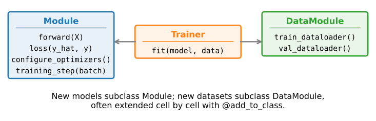
The dataset lives in a DataModule (the object-oriented-design section): where the batches come from, kept separate from the model.

Generating the data

a DataModule that knows the ground truth

A DataModule that builds itself

Generating the data

Draw \mathbf{X}\sim\mathcal{N}(0,1), apply the true line, add tiny noise, all inside __init__ (n=2000 examples, two features):

class SyntheticRegressionData(d2l.DataModule):
    """Synthetic data for linear regression."""
    def __init__(self, w, b, noise=0.01, num_train=1000, num_val=1000, 
                 batch_size=32):
        super().__init__()
        self.save_hyperparameters()
        n = num_train + num_val
        self.X = d2l.randn(n, len(w))
        eps = d2l.randn(n, 1) * noise
        self.y = d2l.matmul(self.X, d2l.reshape(w, (-1, 1))) + b + eps

save_hyperparameters() stores every argument as an attribute.

Fix the ground truth, then peek

Generating the data

Instantiate with the true \mathbf{w}^*=[2,-3.4]^\top, b^*=4.2:

data = SyntheticRegressionData(w=d2l.tensor([2, -3.4]), b=4.2)

Each feature row is a vector in \mathbb{R}^2; each label is a scalar:

print('features:', data.X[0],'\nlabel:', data.y[0])

features: [ 1.2680211 -0.9800729] 
label: [10.066712]

Memorize [2, -3.4] and 4.2: the next two sections train models whose only pass mark is giving these numbers back.

Reading the data

minibatches, by hand and by framework

A minibatch sampler, by hand

Reading the data

Roll the minibatch loader ourselves: shuffle the indices (afresh on every training pass), then yield batch_size rows at a time (one batch is 32\times2 features, 32\times1 labels).

def get_dataloader(self, train):
    if train:
        indices = list(range(0, self.num_train))
        # The examples are read in random order
        random.shuffle(indices)
    else:
        indices = list(range(self.num_train, self.num_train+self.num_val))
    for i in range(0, len(indices), self.batch_size):
        batch_indices = d2l.tensor(indices[i: i+self.batch_size])
        yield self.X[batch_indices], self.y[batch_indices]

Transparent, but it costs three ways: all data in memory, single-threaded Python, and no prefetching to overlap loading with compute.

The built-in loader

same interface, production speed

Hand the work to the framework

The built-in loader

The framework’s loader shuffles, prefetches, and parallelizes for us. Wrap the tensors once…

@d2l.add_to_class(d2l.DataModule)
def get_tensorloader(self, tensors, train, indices=slice(0, None)):
    tensors = tuple(a[indices] for a in tensors)
    dataset = gluon.data.ArrayDataset(*tensors)
    return gluon.data.DataLoader(dataset, self.batch_size,
                                 shuffle=train)

…then rewire get_dataloader to use it (training vs. validation split):

@d2l.add_to_class(SyntheticRegressionData)
def get_dataloader(self, train):
    i = slice(0, self.num_train) if train else slice(self.num_train, None)
    return self.get_tensorloader((self.X, self.y), train, i)

Same interface, drop-in

The built-in loader

The caller sees an identical protocol, one minibatch at a time:

X, y = next(iter(data.train_dataloader()))
print('X shape:', X.shape, '\ny shape:', y.shape)

X shape: (32, 2) 
y shape: (32, 1)

And it knows its own length, so len(dl) is the batches per epoch (\lceil 1000/32\rceil = 32: 31 full, one of 8):

len(data.train_dataloader())

Recap

Wrap-up

Synthetic data fixes the answer up front (\mathbf{w}^*=[2,-3.4], b^*=4.2), so a failed fit can only be the algorithm’s fault.
A DataModule packages where batches come from, reusable across models.

Hand-rolled vs. built-in loader: one protocol; the framework version shuffles, prefetches, parallelizes.
Watch the last batch: a loader either keeps the partial final minibatch or drops it (32 vs. 31 batches here).