The ImageNet Moment: AlexNet

Before 2012: features were crafted

Classical vision pipelines never fed raw pixels to a classifier:

• hand-engineered extractors (SIFT, SURF, bags of visual words) computed the representation;
• a linear model or kernel method handled the final classification.

Progress meant inventing better features, not better learning.

The bet: learn the representation

LeCun, Hinton, Bengio, Ng, Amari, Schmidhuber: features should be learned, hierarchically, layer by layer.

AlexNet’s first layer learned filters that resemble the hand-crafted ones:

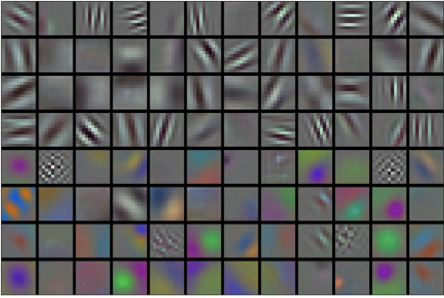
First-layer filters learned by AlexNet.

What changed: data and compute

• ImageNet (2009): 1.2 M labeled images, 1000 classes, 224×224 resolution.
• GPUs: from 1999 to 2012, throughput grew by roughly three orders of magnitude.
• Plus the missing training tricks: ReLU, dropout, augmentation, better initialization.

AlexNet (Krizhevsky, Sutskever, Hinton, 2012) put them together and won ILSVRC 2012 by a large margin.

From LeNet to AlexNet

Same design, scaled up: convolutional stages, then a fully connected head.

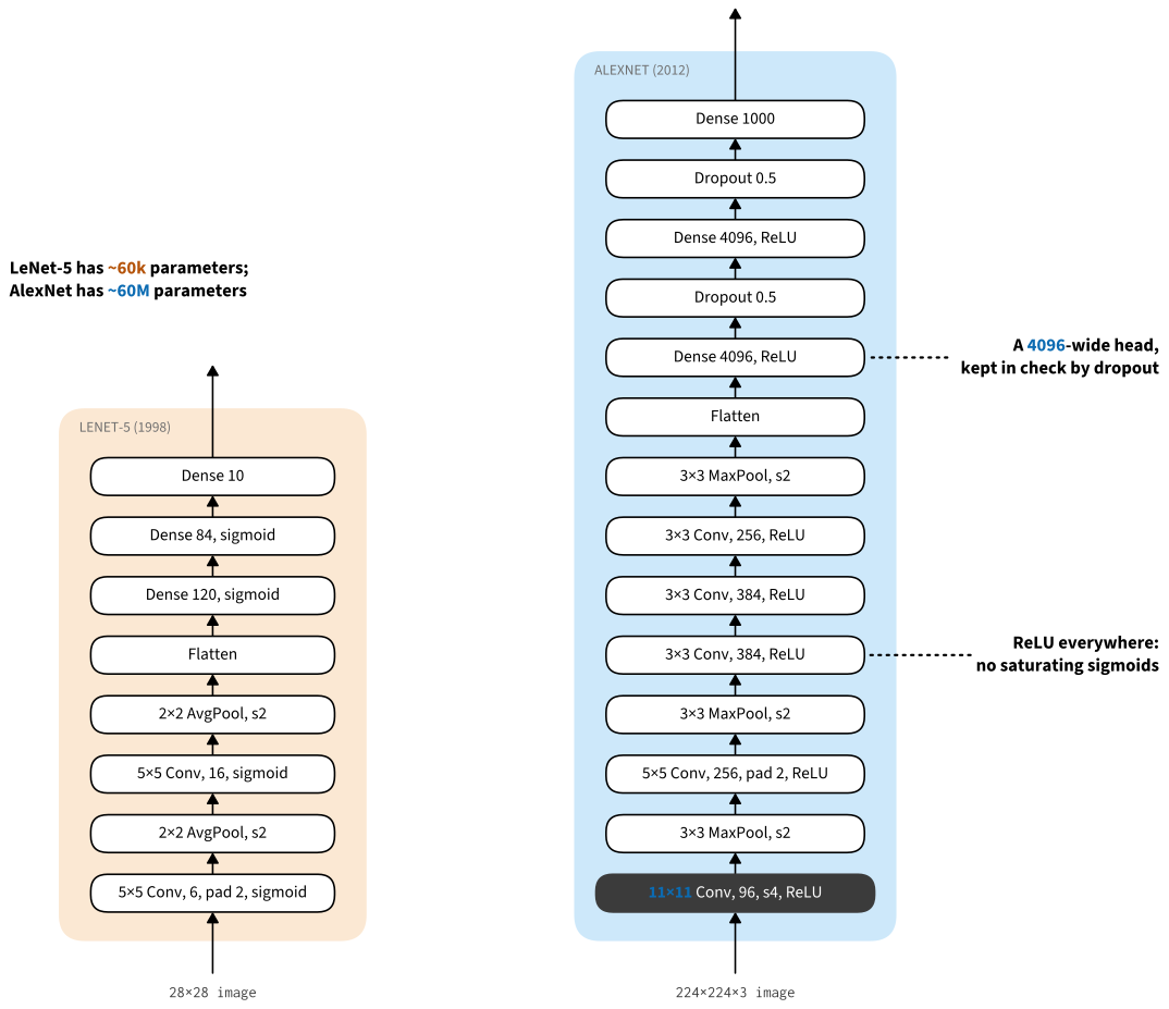
LeNet and AlexNet side by side.

The architecture in code

Five conv layers (11×11 → 5×5 → three 3×3) with max-pooling, then two 4096-wide dense layers with dropout:

from d2l import mxnet as d2l
from mxnet import np, init, npx
from mxnet.gluon import nn
npx.set_np()

class AlexNet(d2l.Classifier):
    def __init__(self, lr=0.1, num_classes=10):
        super().__init__()
        self.save_hyperparameters()
        self.net = nn.Sequential()
        self.net.add(
            nn.Conv2D(96, kernel_size=11, strides=4, activation='relu'),
            nn.MaxPool2D(pool_size=3, strides=2),
            nn.Conv2D(256, kernel_size=5, padding=2, activation='relu'),
            nn.MaxPool2D(pool_size=3, strides=2),
            nn.Conv2D(384, kernel_size=3, padding=1, activation='relu'),
            nn.Conv2D(384, kernel_size=3, padding=1, activation='relu'),
            nn.Conv2D(256, kernel_size=3, padding=1, activation='relu'),
            nn.MaxPool2D(pool_size=3, strides=2),
            nn.Dense(4096, activation='relu'), nn.Dropout(0.5),
            nn.Dense(4096, activation='relu'), nn.Dropout(0.5),
            nn.Dense(num_classes))
        self.net.initialize(init.Xavier())

Shape inspection

Walk a single 224×224 image through the network and print each block’s output shape, from 224×224 down to 6×6 at 256 channels:

AlexNet().layer_summary((1, 1, 224, 224))

Conv2D output shape:     (1, 96, 54, 54)
MaxPool2D output shape:  (1, 96, 26, 26)
Conv2D output shape:     (1, 256, 26, 26)
MaxPool2D output shape:  (1, 256, 12, 12)
Conv2D output shape:     (1, 384, 12, 12)
Conv2D output shape:     (1, 384, 12, 12)
...
MaxPool2D output shape:  (1, 256, 5, 5)
Dense output shape:  (1, 4096)
Dropout output shape:    (1, 4096)
Dense output shape:  (1, 4096)
Dropout output shape:    (1, 4096)
Dense output shape:  (1, 10)

Training on Fashion-MNIST

Upsample the 28×28 Fashion-MNIST images to the 224×224 input AlexNet expects, then train with a smaller learning rate than LeNet:

model = AlexNet(lr=0.01)
data = d2l.FashionMNIST(batch_size=128, resize=(224, 224))
trainer = d2l.Trainer(max_epochs=10, num_gpus=1)
trainer.fit(model, data)

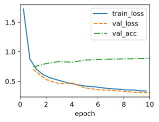
Recap

• AlexNet is LeNet’s recipe at scale: 8 layers, ~60 M parameters, ReLU, dropout, GPU training, ImageNet.
• Learned features displaced a decade of hand-crafted pipelines.
• Its huge dense head is costly; the architectures in the next sections trim it away step by step.