Transposed Convolution

A standard convolution + pooling stack reduces spatial resolution. For dense prediction (semantic segmentation, generative models, super-resolution) we need to go the other way — upsample features back to image resolution.

The standard tool: transposed convolution, also called “deconvolution” (a misnomer — it’s not a true inverse). Each input element broadcasts a full kernel into the output, contributions from neighbors get summed:

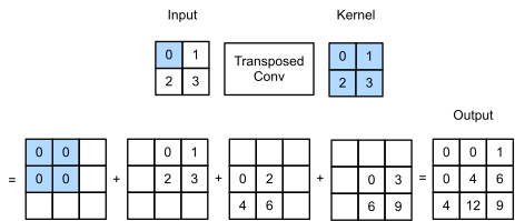
A 2 \times 2 transposed convolution: each input element scatters its kernel into the output.

Output shape grows: with stride 1, kernel k, no padding, n_{\text{out}} = n_{\text{in}} + k - 1. With stride s, multiplied accordingly.

From-scratch implementation

from mxnet import np, npx, init
from mxnet.gluon import nn
from d2l import mxnet as d2l

npx.set_np()

def trans_conv(X, K):
    h, w = K.shape
    Y = d2l.zeros((X.shape[0] + h - 1, X.shape[1] + w - 1))
    for i in range(X.shape[0]):
        for j in range(X.shape[1]):
            Y[i: i + h, j: j + w] += X[i, j] * K
    return Y

Verify on a small example

The hand-written implementation should match the framework operator. If the shape or values differ, the usual culprits are padding semantics or channel layout:

X = d2l.tensor([[0.0, 1.0], [2.0, 3.0]])
K = d2l.tensor([[0.0, 1.0], [2.0, 3.0]])
trans_conv(X, K)

Same result via the framework op (PyTorch ConvTranspose2d, etc.):

X, K = X.reshape(1, 1, 2, 2), K.reshape(1, 1, 2, 2)
tconv = nn.Conv2DTranspose(1, kernel_size=2)
tconv.initialize(init.Constant(K))
tconv(X)

Padding, stride, channels

Padding here removes output rows/columns instead of adding them — it’s the inverse interpretation.

Stride > 1 inserts zeros between input elements before the scatter — that’s how transposed conv upsamples:

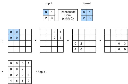
Stride-2 transposed conv: each input element’s kernel is placed at twice-spaced positions, then summed.

tconv = nn.Conv2DTranspose(1, kernel_size=2, padding=1)
tconv.initialize(init.Constant(K))
tconv(X)

tconv = nn.Conv2DTranspose(1, kernel_size=2, strides=2)
tconv.initialize(init.Constant(K))
tconv(X)

Multi-channel works as expected: input channels reduce-add through the kernel, output channels stack in parallel:

X = np.random.uniform(size=(1, 10, 16, 16))
conv = nn.Conv2D(20, kernel_size=5, padding=2, strides=3)
tconv = nn.Conv2DTranspose(10, kernel_size=5, padding=2, strides=3)
conv.initialize()
tconv.initialize()
tconv(conv(X)).shape == X.shape

Connection to matrix transposition

A standard convolution can be written as a sparse matrix multiplication \mathbf{y} = \mathbf{K}\mathbf{x} where \mathbf{K} encodes the kernel + stride + padding.

A transposed convolution multiplies by the transpose: \mathbf{x}' = \mathbf{K}^\top \mathbf{y}. That’s where the name comes from.

X = d2l.reshape(d2l.arange(9.0), (3, 3))
K = d2l.tensor([[1.0, 2.0], [3.0, 4.0]])
Y = d2l.corr2d(X, K)
Y

def kernel2matrix(K):
    k, W = d2l.zeros(5), d2l.zeros((4, 9))
    k[:2], k[3:5] = K[0, :], K[1, :]
    W[0, :5], W[1, 1:6], W[2, 3:8], W[3, 4:] = k, k, k, k
    return W

W = kernel2matrix(K)
W

Matrix view (cont.)

Y == d2l.reshape(d2l.matmul(W, d2l.reshape(X, (-1, 1))), (2, 2))

Z = trans_conv(Y, K)
Z == d2l.reshape(d2l.matmul(d2l.transpose(W), d2l.reshape(Y, (-1, 1))), (3, 3))

Recap

Transposed conv = upsampling op; each input element scatters a full kernel into the output and overlapping contributions sum.
Stride > 1 inserts zeros between inputs → upsamples by s.
Mathematically the transpose of a normal convolution’s matrix form (hence the name).
Workhorse for FCN, U-Net, GAN generators, VAE decoders.
Modern alternative: bilinear upsample + 3×3 conv — avoids checkerboard artifacts that transposed conv can produce.