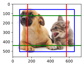
%matplotlib inline
from d2l import mxnet as d2l
from mxnet import image, np, npx

npx.set_np()

img = image.imread('../img/catdog.jpg')
h, w = img.shape[:2]
h, wSmall objects on a fine map
4 \times 4 feature map, small anchor scale → dense coverage of small image regions. Notice the many anchor centers: that density is what small objects need.
display_anchors(fmap_w=4, fmap_h=4, s=[0.15])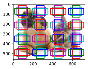
Medium objects on a coarser map
2 \times 2 feature map, larger anchor scale — fewer anchors, each covering more area:
display_anchors(fmap_w=2, fmap_h=2, s=[0.4])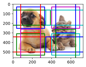
Large objects on the coarsest map
1 \times 1 feature map, anchor scale 0.8 — the whole image as a single anchor, with several aspect ratios. This level cannot localize tiny details, but it matches objects that occupy most of the image.
display_anchors(fmap_w=1, fmap_h=1, s=[0.8])