class LSTMScratch(nnx.Module):
    """The long short-term memory (LSTM) cell implemented from scratch."""
    def __init__(self, num_inputs, num_hiddens, sigma=0.01, rngs=None):
        rngs = nnx.Rngs(0) if rngs is None else rngs
        self.num_inputs, self.num_hiddens = num_inputs, num_hiddens
        self.sigma = sigma
        init_weight = lambda shape: nnx.Param(
            rngs.params.normal(shape) * sigma)
        triple = lambda: (
            init_weight((num_inputs, num_hiddens)),
            init_weight((num_hiddens, num_hiddens)),
            nnx.Param(jnp.zeros(num_hiddens)))
        self.W_xi, self.W_hi, self.b_i = triple()  # Input gate
        self.W_xf, self.W_hf, self.b_f = triple()  # Forget gate
        self.W_xo, self.W_ho, self.b_o = triple()  # Output gate
self.W_xc, self.W_hc, self.b_c = triple() # Input nodeThe LSTM memory cell
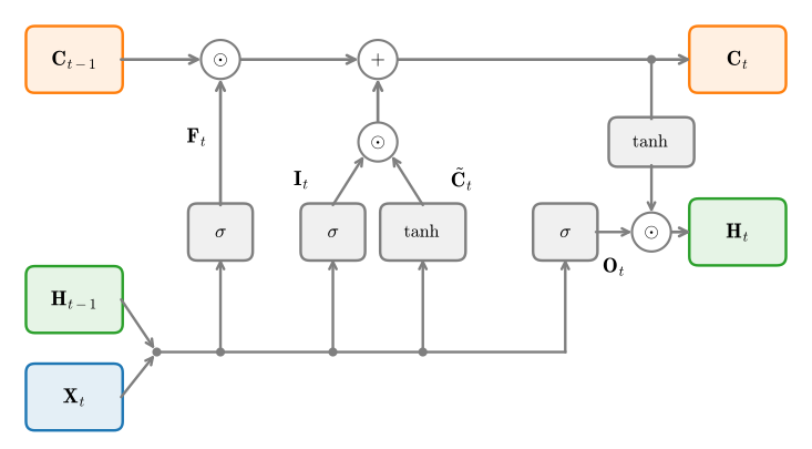
The cell state is touched only by an elementwise product and a sum; gates control write, keep, and reveal.
Training on The Time Machine
Same recipe as the vanilla RNN (50k windows of 32 BPE tokens, batch 1024, emb 64, hidden 128, 10 epochs, clip 1), so the numbers are directly comparable:
data = d2l.TimeMachine(batch_size=1024, num_steps=32,
                       num_train=50000, num_val=5000)
lstm = LSTMScratch(num_inputs=64, num_hiddens=128)
model = d2l.RNNLMScratch(lstm, vocab_size=len(data.vocab), lr=4)trainer = d2l.Trainer(max_epochs=10, gradient_clip_val=1, num_gpus=1)
model.board.yscale = 'log'
trainer.fit(model, data)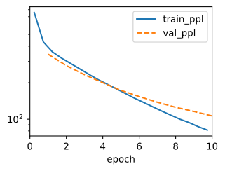
Train and generate
lstm = LSTM(num_inputs=64, num_hiddens=128)
model = d2l.RNNLM(lstm, vocab_size=len(data.vocab), lr=4)trainer = d2l.Trainer(max_epochs=10, gradient_clip_val=1, num_gpus=1)
model.board.yscale = 'log'
trainer.fit(model, data)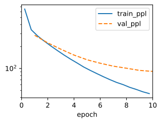
ppls['LSTM'] = val_ppl(model)
pred = model.predict('the time traveller', 30, data.tokenizer,
temperature=0.5)
d2l.print_wrapped(f"perplexity {ppls['LSTM']:.1f}, {pred!r}")perplexity 93.1, 'the time travellering a fair\nof trailing to the Palace of
the hall, and now, but\nI could see, I'GRU: two gates, no cell
Cho et al. (2014): drop the separate cell state, merge to two gates.
\tilde{\mathbf{H}}_t = \tanh(\mathbf{X}_t \mathbf{W}_{xh} + (\mathbf{R}_t \odot \mathbf{H}_{t-1}) \mathbf{W}_{hh} + \mathbf{b}_h), \mathbf{H}_t = \mathbf{Z}_t \odot \mathbf{H}_{t-1} + (1 - \mathbf{Z}_t) \odot \tilde{\mathbf{H}}_t.
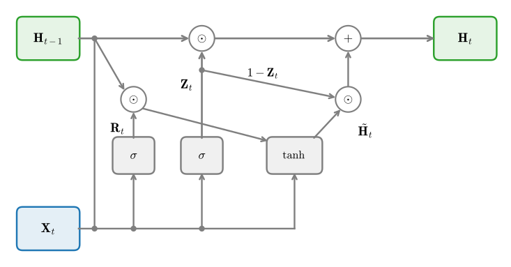
Reset gates the past inside the candidate; update convex-blends old and new.
GRU in code
class GRU(d2l.RNN):
"""The multilayer GRU model implemented with high-level APIs."""
def __init__(self, num_inputs, num_hiddens, num_layers=1, dropout=0,
rngs=None):
rngs = nnx.Rngs(params=0, dropout=1, carry=2) if rngs is None \
else rngs
self.num_inputs, self.num_hiddens = num_inputs, num_hiddens
self.num_layers = num_layers
self.rnns = nnx.List([
nnx.RNN(nnx.GRUCell(num_inputs if i == 0 else num_hiddens,
num_hiddens, rngs=rngs),
time_major=True, return_carry=True, rngs=rngs)
for i in range(num_layers)])
self.dropouts = nnx.List([
nnx.Dropout(dropout, rngs=rngs) for _ in range(num_layers - 1)])
def __call__(self, X, state=None):
outputs = X
state = [None] * self.num_layers if state is None else state
new_state = []
for i, rnn in enumerate(self.rnns):
carry, outputs = rnn(outputs, initial_carry=state[i])
new_state.append(carry)
if i < self.num_layers - 1:
outputs = self.dropouts[i](outputs)
return outputs, new_stategru = GRU(num_inputs=64, num_hiddens=128)
model = d2l.RNNLM(gru, vocab_size=len(data.vocab), lr=4)trainer = d2l.Trainer(max_epochs=10, gradient_clip_val=1, num_gpus=1)
model.board.yscale = 'log'
trainer.fit(model, data)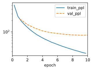
ppls['GRU'] = val_ppl(model)
print(f"validation perplexity {ppls['GRU']:.1f}")validation perplexity 81.8Three quarters of the LSTM’s recurrent parameters and the best perplexity in this section’s runs: fewer gates converge faster on a short budget. Its 2020s legacy: strip the gates to input-only functions and the recurrence turns linear → minGRU, LRU, SSMs.
Depth and direction, briefly
Layer l reads layer l{-}1 at the same step and itself at the previous step; a one-argument change with num_layers:
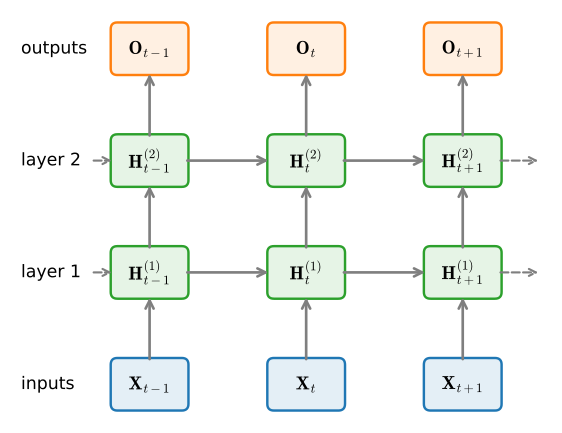
lstm2 = LSTM(num_inputs=64, num_hiddens=128, num_layers=2)
model = d2l.RNNLM(lstm2, vocab_size=len(data.vocab), lr=4)
trainer = d2l.Trainer(max_epochs=10, gradient_clip_val=1, num_gpus=1)
model.board.yscale = 'log'
trainer.fit(model, data)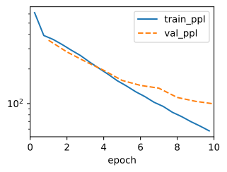
ppls['LSTM (2 layers)'] = val_ppl(model)
print(f'{"model":>16} {"val ppl":>8}')
for name, p in ppls.items():
    print(f'{name:>16} {p:>8.1f}')
model val ppl
LSTM (scratch) 103.8
LSTM 93.1
GRU 81.8
LSTM (2 layers) 98.2On this small corpus, the second layer does not improve the result. Additional depth is useful only when the data and optimization support it.
Bidirectional RNNs
Two chains, one forward and one backward, concatenated per step, so every output conditions on the whole sequence:
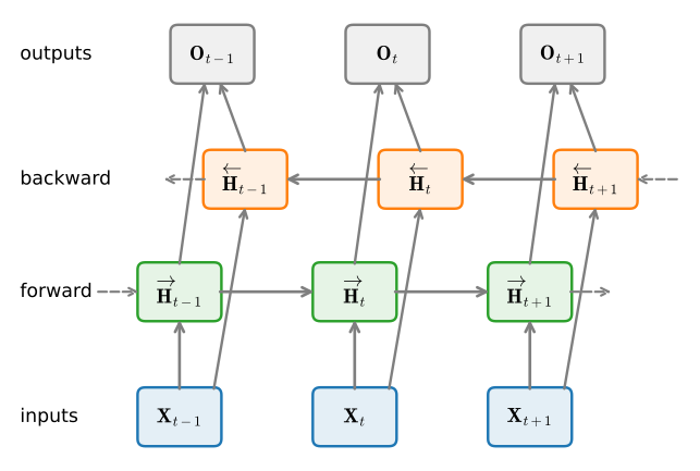
Forward + backward chains, outputs read 2h features.
birnn = nnx.Bidirectional(
    nnx.RNN(nnx.LSTMCell(64, 128, rngs=nnx.Rngs(0)),
            time_major=True, rngs=nnx.Rngs(0)),
    nnx.RNN(nnx.LSTMCell(64, 128, rngs=nnx.Rngs(1)), time_major=True,
            reverse=True, keep_order=True, rngs=nnx.Rngs(1)),
    time_major=True)
X = jax.random.normal(d2l.get_key(), (32, 8, 64))
outputs = birnn(X)
outputs.shape
(32, 8, 256)No use unchanged as a causal decoder: at sampling time the future does not exist; “next-token training” hands the model the answer. Use for tagging/encoding (ELMo → BERT); fine inside generative systems as the encoder.