def delta_recurrent(Q, K, V, beta):
"""The delta rule in the error form: read, subtract, write, read out."""
def step(S, qkvb):
q, k, v, b = qkvb
error = v - S.T @ k # What the memory got wrong
S = S + b * k[:, None] * error[None, :]
return S, S.T @ q
S0 = jnp.zeros((Q.shape[-1], V.shape[-1]))
return jax.lax.scan(step, S0, (Q, K, V, beta))[1]
def delta_recurrent_matrix(Q, K, V, beta):
"""The same update as transition-then-write, for the family template."""
def step(S, qkvb):
q, k, v, b = qkvb
S = (jnp.eye(len(k)) - b * jnp.outer(k, k)) @ S + b * jnp.outer(k, v)
return S, S.T @ q
S0 = jnp.zeros((Q.shape[-1], V.shape[-1]))
return jax.lax.scan(step, S0, (Q, K, V, beta))[1]
d_k, d_v, T = 64, 64, 512
rng_keys = jax.random.split(jax.random.key(0), 4)
Q, K, V = (jax.random.normal(k, (T, d))
for k, d in zip(rng_keys, (d_k, d_k, d_v)))
K = K / jnp.maximum(jnp.linalg.norm(K, axis=-1, keepdims=True),
1e-12) # Unit keys; F.normalize contract
beta = jax.nn.sigmoid(jax.random.normal(rng_keys[3], (T,)))
with jax.default_matmul_precision('highest'):
y_delta = delta_recurrent(Q, K, V, beta)
err = jnp.abs(y_delta - delta_recurrent_matrix(Q, K, V, beta)).max() \
/ jnp.abs(y_delta).max()
print(f'error form vs matrix form: relative deviation {float(err):.2e}')
assert err < 1e-5 # One rule, two readingsDeltaNet and Corrective Memory Updates
Dive into Deep Learning · §12.5
DeltaNet
memory that edits: the overwrite failure · one SGD step per token · the WY trick · Gated DeltaNet · what a transition can compute
Additive Write Rules
Last section’s family table: seven models, three lineages — and every write is an addition.
- Decay manages crowding; it discounts by age.
- But streams re-bind: the same ticker, a reassigned variable, a character who moves. Staleness is indexed by key.
After R writes to one key: \mathbf{S}^\top \mathbf{k} = \mathbf{v}^{(1)} + \cdots + \mathbf{v}^{(R)} — the current and stale bindings receive the same weight.
Overwriting, measured
8 orthonormal keys (zero cross-key interference by construction), R shuffled re-bindings per key, read back the latest:
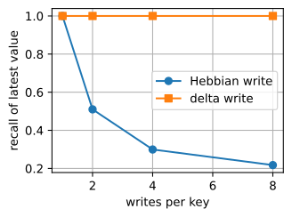
writes/key   Hebbian   delta
         1     1.000   1.000
         2     0.510   1.000
         4     0.299   1.000
8 0.217 1.000- Hebbian: recall \approx guessing among the R superposed values.
- Erase-then-write: 1.000 at every R — the last write always wins.
Trained models hit the same ceiling
Same task, end-to-end training, identical parameter counts; only the write line differs:
writes/key   Hebbian   delta
         1     1.000   1.000
         2     0.531   1.000
         4     0.327   1.000
         6     0.265   1.000
Design constraint (learned the hard way): the write address (q, k, \beta) must come from the key token alone — give it the value token and a Hebbian model escapes by assigning every pair its own address.
The delta rule
One SGD step on the recall loss makes the state predict the target value, rather than only increasing alignment:
\ell_t(\mathbf{S}) = \tfrac{1}{2}\|\mathbf{S}^\top \mathbf{k}_t - \mathbf{v}_t\|^2, \qquad \mathbf{S}_t = \mathbf{S}_{t-1} - \beta_t\, \mathbf{k}_t (\mathbf{k}_t^\top \mathbf{S}_{t-1} - \mathbf{v}_t^\top)
- Widrow–Hoff 1960 → fast weight programmers (Schlag et al. 2021) → parallel DeltaNet (Yang et al. 2024).
- Hebbian write = SGD on -\langle \mathbf{S}^\top\mathbf{k}_t, \mathbf{v}_t\rangle: alignment, no feedback — that is the whole difference.
Unit key: stored value moves to (1-\beta_t)\mathbf{v}_{\textrm{old}} + \beta_t \mathbf{v}_t — \beta is a learned write strength (a per-token learning rate).
One rule, two readings
error form vs matrix form: relative deviation 1.38e-06- Error form: two matrix–vector products per token — the algorithm.
- Matrix form: transition \mathbf{I} - \beta_t \mathbf{k}_t\mathbf{k}_t^\top + write — the family template.
Training it: the WY trick
Transitions are no longer diagonal — no segsum. But within a chunk the updates couple only through key overlaps:
(\mathbf{I} + \mathbf{A})\,\mathbf{U} = \mathrm{diag}(\boldsymbol{\beta})(\mathbf{V} - \mathbf{K}\mathbf{S}), \qquad A_{ts} = \beta_t\,\mathbf{k}_t^\top \mathbf{k}_s,\; s < t
One unit-triangular solve per chunk, against the actual right-hand side — \mathcal{O}(C^2 d_v), never form the inverse; then attention inside, recurrence across, as before.
chunk size   16: relative deviation 3.46e-07
chunk size   64: relative deviation 4.32e-07
chunk size  256: relative deviation 4.76e-07
Production kernels: the flash-linear-attention library — same algorithm.
Gating: the modern cell
DeltaNet preserves every unwritten row exactly — stale rows never fade. Add back a decay, decoupled from the write:
\mathbf{S}_t = \alpha_t\big(\mathbf{I} - \beta_t \mathbf{k}_t\mathbf{k}_t^\top\big)\mathbf{S}_{t-1} + \beta_t\,\mathbf{k}_t\mathbf{v}_t^\top
- \beta_t = learning rate, \alpha_t = weight decay, applied decoupled — the gate plays AdamW’s decoupled-decay role (that one axis; no moments, no bias corrections).
- \beta_t = 0: Mamba-2’s row. \alpha_t = 1: pure DeltaNet.
- Shipped: Qwen3-Next (Gated DeltaNet), Kimi Linear (KDA), RWKV-7’s line.
On the scoreboard
Same capstone recipe as the Mamba row — The Time Machine, 50k windows, ten epochs:
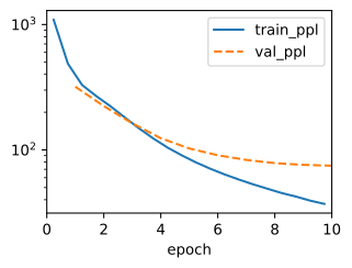
          model  val ppl    params  s/epoch
Gated DeltaNet 74.5 562,315 4.4- Lands in the strongest band of the chapter’s scoreboard at comparable parameter count.
- At 1.3B scale: Gated DeltaNet beats Mamba-2 and DeltaNet — decay without delta trails on recall; delta without decay trails on modeling.
The generalized delta rule
RWKV-7 decouples every role the delta rule ties together:
\mathbf{S}_t = \big(\mathrm{diag}(\mathbf{w}_t) - (\mathbf{a}_t \odot \hat{\boldsymbol{\kappa}}_t)\,\hat{\boldsymbol{\kappa}}_t^\top\big)\,\mathbf{S}_{t-1} + \tilde{\mathbf{k}}_t\mathbf{v}_t^\top
- Per-channel decay \mathbf{w}_t · removal key \hat{\boldsymbol{\kappa}}_t ≠ write key \tilde{\mathbf{k}}_t · per-channel write rate \mathbf{a}_t.
- Tie them all → DeltaNet exactly (asserted in the notebook).
The family now has two parents: decay structure × write rule.
What the transition can compute: parity
Purely multiplicative recurrence \mathbf{h}_t = \mathbf{a}_t \odot \mathbf{h}_{t-1}; the only difference is the range of \mathbf{a}_t:
T= 8  sigmoid, a in (0,1): 0.512  0.697  0.375
T= 8  tanh,    a in (-1,1): 1.000  1.000  1.000
T=16  sigmoid, a in (0,1): 0.486  0.486  0.496
T=16  tanh,    a in (-1,1): 0.487  1.000  1.000
T=24  sigmoid, a in (0,1): 0.483  0.483  0.483
T=24 tanh, a in (-1,1): 0.483 1.000 1.000- (0,1): chance in every run — a representational wall: the dynamics cannot flip a sign.
- (-1,1): every seed solves it at T=8; longer T = an optimization horizon, failing seeds from T=16 on.
The Reflection in the Delta Rule
\mathbf{I} - \beta\,\mathbf{k}\mathbf{k}^\top has eigenvalue 1 - \beta along \mathbf{k}:
beta = 0.5: eigenvalues +0.5 (along k), +1.0 (elsewhere)
beta = 1.0: eigenvalues -0.0 (along k), +1.0 (elsewhere)
beta = 1.5: eigenvalues -0.5 (along k), +1.0 (elsewhere)
beta = 2.0: eigenvalues -1.0 (along k), +1.0 (elsewhere)
T =  8, beta = 1 (projection): parity accuracy 0.529
T =  8, beta = 2 (reflection): parity accuracy 1.000
T = 24, beta = 1 (projection): parity accuracy 0.518
T = 24, beta = 2 (reflection): parity accuracy 1.000
T = 64, beta = 1 (projection): parity accuracy 0.501
T = 64, beta = 2 (reflection): parity accuracy 1.000- \beta = 1: projection — erases, parity lost. \beta = 2: reflection — exact at T = 64, nothing optimized.
- That one eigenvalue is the flag
allow_neg_eigval: double the gate to 2\sigma(\cdot) \in (0, 2) (Grazzi et al. 2025) — open interval, so \beta = 2 itself is the boundary construction.
Transition Structure Determines Representable Dynamics
| transition | unlocks |
|---|---|
| scalar / diagonal (0,1) | forgetting; parity out of reach |
| diagonal (-1,1) | parity |
| Householder, \beta \in (0,2) | targeted edits + reflections |
| product of n_h Householders | group word problems (DeltaProduct) |
| dense nonlinear | S_5 and beyond — at sequential cost |
- The \mathsf{TC}^0 ceiling (Merrill et al. 2024): diagonal SSMs and transformers share it — an “illusion of state.”
The state remains fixed-size and less expressive than a nonlinear recurrence. Hybrid architectures address the capacity gap. The next section first interprets a sequence layer as an optimizer.