num_tosses = 100
heads = sum([random.random() > 0.5 for _ in range(num_tosses)])
tails = num_tosses - heads
print("heads, tails: ", [heads, tails])Probability and Statistics
Dive into Deep Learning · §1.6
Reasoning under uncertainty
sampling · distributions · Bayes · expectation
Machine learning is inference under uncertainty
Motivation
- A model rarely returns one answer: it returns a distribution over answers.
- Many training objectives derive from likelihoods, often through a negative log-likelihood.
- Generalization, regularization, and the Bayesian view all rest on the same handful of rules.
Probability reasons forward: model → data. Statistics reasons backward: data → model. We build both, on one running example.
01
From data to a probability
sampling, frequencies, the law of large numbers
A coin of unknown bias
Estimating from data
We find a coin and want P(\text{heads}), but nobody tells us its value. The plan: toss it many times and count.
A single batch of 100 tosses with random.random() often lands near 50/50, but need not do so exactly because sampling has variance:
heads, tails: [40, 60]Multinomial draws 100 tosses in one call
Estimating from data
A Multinomial over {heads, tails} with probabilities [0.5, 0.5] returns the count vector directly:
Array([35, 65], dtype=int32)More data, tighter estimate
Estimating from data
With 10,000 tosses the frequencies are typically closer to the true \tfrac{1}{2}:
Array([0.4974, 0.5026], dtype=float32)The law of large numbers: as the number of trials n \to \infty, the empirical frequency converges to the true probability.
The estimate converges at a 1/√n rate
Estimating from data
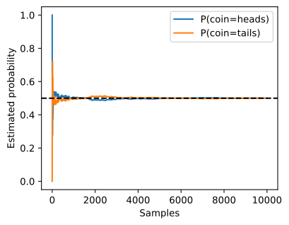
The running estimate settles toward 0.5 as the sample count grows:
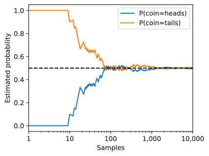
The error shrinks like 1/\sqrt{n}: to halve it you need 4× the data.
A first glimpse of the real question of statistics: how sure we are of what we estimate.
The 1/√n law, measured: slope −½
Estimating from data
Why 1/\sqrt{n}? Each toss has variance p(1-p); averaging n independent tosses gives
\textrm{Var}[\hat{p}] = \frac{p(1-p)}{n}.
Estimating p from 1000 batches at each n, the standard deviation of the estimates follows the predicted 0.5/\sqrt{n} line: slope -\tfrac12 on log–log axes.
02
The formal language
sample spaces, events, random variables
Three axioms determine the probability calculus
Formal treatment
Every outcome lives in a sample space \mathcal{S}; an event is a measurable subset. A probability assigns each event a number in [0,1] obeying three rules (Kolmogorov):
- P(\mathcal{A}) \ge 0;
- P(\mathcal{S}) = 1;
- disjoint events add.
Standard identities follow from them; for example, inclusion–exclusion gives P(\mathcal{A}\cup\mathcal{B}) = P(\mathcal{A}) + P(\mathcal{B}) - P(\mathcal{A}\cap\mathcal{B}).
Mass sits on points; density needs intervals
Formal treatment
A random variable maps outcomes to values. Discrete ones (a die) place mass on points; continuous ones (a height) spread density along the line.
For a continuous variable an exact value has probability zero: only intervals carry probability, obtained by integrating the density.
03
Joint, marginal, conditional
how two variables relate, and Bayes’ theorem
A joint table yields marginals and conditionals
Multiple variables
The joint P(A,B) lists every combination. From it:
- sum a row or column → a marginal P(A) or P(B);
- renormalize one row → a conditional P(B \mid A{=}a) = \dfrac{P(A{=}a,\, B)}{P(A{=}a)}.
Conditioning = restrict to the slice where A{=}a, then rescale so it sums to 1.
Bayes’ theorem reverses the conditioning
Multiple variables
Write the joint two ways, P(A,B) = P(B\mid A)\,P(A) = P(A\mid B)\,P(B), and equate:
P(A \mid B) = \frac{P(B \mid A)\,P(A)}{P(B)}.
This converts P(B \mid A) into the reverse conditional needed to infer a cause A from an effect B.
posterior \propto likelihood \times prior: \;P(H \mid E) \propto P(E \mid H)\,P(H).
Independence, and explaining away
Multiple variables
Independence, A \perp B, means P(A,B) = P(A)\,P(B). But conditioning changes dependence: a common cause links two variables until you condition on it; a collider (common effect) makes independent causes dependent once you do: explaining away.
04
Bayes in action: the HIV test
why a “99% accurate” test can still mislead
A test that never misses can still mislead
Worked example
The test catches every true HIV case but has a 1% false-positive rate, and the disease is rare:
\begin{aligned} P(D{=}1 \mid H{=}1) &= 1.00 \\ P(D{=}1 \mid H{=}0) &= 0.01 \\ \text{prior } P(H{=}1) &= 0.0015 \end{aligned}
We want the posterior P(H{=}1 \mid D{=}1). Natural frequencies make the effect of the low base rate explicit.
Of ~115 positives, only 15 are real
Worked example
Among 10,000 people only ~15 truly have HIV, but ~100 healthy people also test positive:
P(H{=}1 \mid D{=}1) \approx \tfrac{15}{115} \approx 13\%.
The low base rate keeps the posterior well below the test’s sensitivity.
A second positive: 0.15% → 13% → 83%
Worked example
A second, independent positive test multiplies the evidence: applying Bayes again drives the posterior from the 0.15\% prior to 13\%, then to 83\%.
A simulation of two million patients gives a coarse check of the exact 0.8307; its Monte Carlo standard error is about 0.006:
Array(0.82513815, dtype=float32)05
Summarizing a distribution
expectation, variance, covariance
Expectation: the probability-weighted average
Summaries
E[X] = \sum_x x\,P(X{=}x).
It is the balance point of the distribution. For an investment paying 0, 2\times, or 10\times with probabilities 0.5, 0.4, 0.1, the expected return is 1.8\times.
Variance: same mean, different risk
Summaries
\textrm{Var}[X] = E\big[(X - E[X])^2\big] = E[X^2] - E[X]^2.
Two investments can share a mean yet differ wildly in spread. The standard deviation \sigma = \sqrt{\textrm{Var}[X]} reports it in the original units.
Covariance: the sign says how they move
Summaries
Covariance is the expected product of the two centered variables; its sign says whether they move together (magnitude is scale-dependent; rescale by the standard deviations to get the correlation). Stacked over a vector, it becomes the covariance matrix \boldsymbol{\Sigma}, which is symmetric and recurs in later chapters:
06
Uncertainty & guarantees
what kind, and how far can it stray?
Two kinds of uncertainty
Discussion
Aleatoric uncertainty is intrinsic randomness: the next fair-coin flip stays 50/50 no matter how much data you gather. Epistemic uncertainty is about unknown parameters, and it shrinks as data accumulates.
Tail bounds: guarantees without the distribution
Discussion
Even without knowing the distribution, we can bound how often a nonnegative variable lands far out. Markov: P(X \ge a) \le \frac{E[X]}{a}.
Apply it to (X-\mu)^2 to get Chebyshev; sharper bounds (Hoeffding, Bernstein) and their consequences for generalization are developed in the concentration-and-generalization section.
Recap
Wrap-up
- Sample → count → estimate; the LLN converges at 1/\sqrt{n} (slope -\tfrac12, measured).
- Axioms generate every rule; events combine by inclusion–exclusion.
- The joint yields marginals (sum) and conditionals (renormalize).
- Bayes reverses conditioning: posterior \propto likelihood \times prior.
- Base rates rule rare-disease tests: 13\% after one positive, 0.8307 after two.
- Expectation / variance / covariance summarize a distribution.
- Tail bounds (Markov → Chebyshev) guarantee concentration even when the distribution is unknown.