%matplotlib inline
from d2l import jax as d2l
import jax
from jax import numpy as jnp
import mathSGD trajectory
With a constant learning rate, SGD does not converge to one point. Near the minimum, the true gradient vanishes but sampling noise remains, so the iterates fluctuate around the optimum:
def constant_lr():
    return 1

eta = 0.1
lr = constant_lr  # Constant learning rate
d2l.show_trace_2d(f, d2l.train_2d(sgd, steps=50, f_grad=f_grad))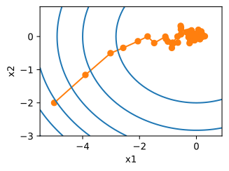
epoch 50, x1: -0.141533, x2: -0.069805Limitation of exponential decay
When \sum_t \eta(t) < \infty, the total possible movement is finite. The iterate may therefore stop short of the optimum:
def exponential_lr():
    # Global variable that is defined outside this function and updated inside
    global t
    t += 1
    return math.exp(-0.1 * t)

t = 1
lr = exponential_lr
d2l.show_trace_2d(f, d2l.train_2d(sgd, steps=1000, f_grad=f_grad))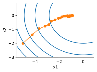
epoch 1000, x1: -0.810909, x2: -0.028332Polynomial decay
\eta(t) \propto t^{-1/2} keeps exploring long enough and converges much better after only 50 steps:
def polynomial_lr():
    # Global variable that is defined outside this function and updated inside
    global t
    t += 1
    return (1 + 0.1 * t) ** (-0.5)

t = 1
lr = polynomial_lr
d2l.show_trace_2d(f, d2l.train_2d(sgd, steps=50, f_grad=f_grad))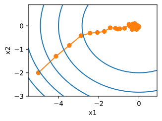
epoch 50, x1: 0.037837, x2: 0.002780Gradient variance vs batch size
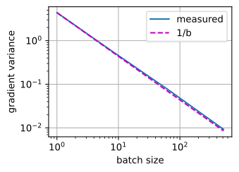
In real training the noise comes from which examples land in the minibatch. Averaging b independent example gradients divides the variance by b. Measured on a real network (2-layer MLP, airfoil data), it holds from batch size 1 to 512:
data_iter, feature_dim = d2l.get_data_ch11(batch_size=10)
X = jnp.concatenate([jnp.asarray(Xb) for Xb, yb in data_iter])
y = jnp.concatenate([jnp.asarray(yb) for Xb, yb in data_iter])

k1, k2 = jax.random.split(jax.random.PRNGKey(1))
params = dict(W1=0.1 * jax.random.normal(k1, (feature_dim, 64)),
              b1=jnp.zeros(64),
              W2=0.1 * jax.random.normal(k2, (64, 1)), b2=jnp.zeros(1))

def batch_loss(params, idx):
    h = jax.nn.relu(X[idx] @ params['W1'] + params['b1'])
    return jnp.mean(((h @ params['W2'] + params['b2']).squeeze()
                     - y[idx]) ** 2) / 2

def batch_grad(idx):  # Flattened loss gradient on the minibatch X[idx]
    grads = jax.grad(batch_loss)(params, idx)
    return jnp.concatenate([g.reshape(-1) for g in jax.tree.leaves(grads)])

g_full = batch_grad(jnp.arange(len(y)))
batch_sizes = [1, 8, 64, 512]
var, key = [], jax.random.PRNGKey(0)
for b in batch_sizes:
    key, subkey = jax.random.split(key)
    idx = jax.random.randint(subkey, (200, b), 0, len(y))
    err = jax.vmap(lambda i: ((batch_grad(i) - g_full) ** 2).sum())(idx)
    var.append(float(err.mean()))
d2l.plot(batch_sizes, [var, [var[0] / b for b in batch_sizes]],
         'batch size', 'gradient variance', xscale='log', yscale='log',
         legend=['measured', '1/b'])