Momentum

Gradient descent has no memory — and pays for it whenever directions disagree about step size.

Ill-conditioned valley: steep walls cap \eta, flat floor needs big \eta. One knob, two masters.
Fix: a running (leaky) average of past gradients — the velocity.
One buffer, one hyperparameter \beta; inside nearly every deep learning optimizer.

An ill-conditioned valley

f(x_1, x_2) = 0.1 x_1^2 + 2 x_2^2 — curvatures 0.2 vs 4:

eta = 0.4
def f_2d(x1, x2):  # Objective
    return 0.1 * x1 ** 2 + 2 * x2 ** 2
def f_2d_grad(x1, x2):  # Gradient of the objective
    return (0.2 * x1, 4 * x2)
def gd_2d(x1, x2, s1, s2, f_grad):
    g1, g2 = f_grad(x1, x2)
    return (x1 - eta * g1, x2 - eta * g2, 0, 0)

d2l.show_trace_2d(f_2d, d2l.train_2d(gd_2d, f_grad=f_2d_grad))

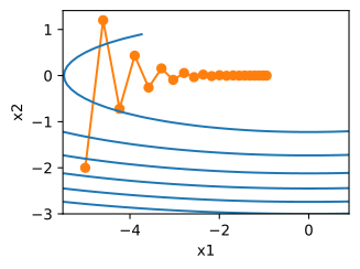
epoch 20, x1: -0.943467, x2: -0.000073

Raise \eta from 0.4 to 0.6: x_1 speeds up, x_2 diverges:

eta = 0.6
d2l.show_trace_2d(f_2d, d2l.train_2d(gd_2d, f_grad=f_2d_grad))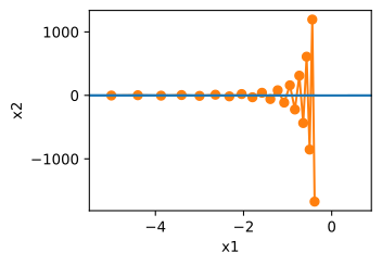

epoch 20, x1: -0.387814, x2: -1673.365109

Leaky averages

Replace the gradient by a velocity:

\mathbf{v}_t = \beta \mathbf{v}_{t-1} + \mathbf{g}_t,\qquad \mathbf{x}_t = \mathbf{x}_{t-1} - \eta \mathbf{v}_t.

Unrolled: \mathbf{v}_t = \sum_{\tau} \beta^{\tau} \mathbf{g}_{t-\tau} — an exponentially weighted sum of the past.

Components that agree accumulate (up to \tfrac{1}{1-\beta}\times).
Components that alternate cancel.
Heavy ball rolling downhill; friction 1-\beta (Polyak, 1964).

Momentum in the valley

Same \eta = 0.6 that just diverged, now with \beta = 0.5:

def momentum_2d(x1, x2, v1, v2, f_grad):
    g1, g2 = f_grad(x1, x2)
    v1, v2 = beta * v1 + g1, beta * v2 + g2
    return x1 - eta * v1, x2 - eta * v2, v1, v2

eta, beta = 0.6, 0.5
d2l.show_trace_2d(f_2d, d2l.train_2d(momentum_2d, f_grad=f_2d_grad))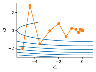

epoch 20, x1: 0.007188, x2: 0.002553

\beta = 0.25: weaker, barely converges — still beats divergence:

eta, beta = 0.6, 0.25
d2l.show_trace_2d(f_2d, d2l.train_2d(momentum_2d, f_grad=f_2d_grad))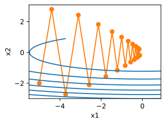

epoch 20, x1: -0.126340, x2: -0.186632

The timescale of β

Weights sum to \tfrac{1}{1-\beta}: momentum \beta ≈ average over the last \tfrac{1}{1-\beta} gradients. \beta=0.9 → ~10 steps; \beta=0.99 → ~100.

d2l.set_figsize()
x = d2l.numpy(d2l.arange(40))
for beta in [0.95, 0.9, 0.6, 0]:
    d2l.plt.plot(x, beta ** x, label=f'beta = {beta:.2f}')
d2l.plt.xlabel('time')
d2l.plt.legend();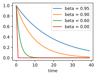

Effective step in persistent directions: \eta / (1-\beta) — raise \beta, lower \eta.

Acceleration: the √κ law

Quadratic with condition number \kappa:

Gradient descent: \mathcal{O}(\kappa \log \tfrac{1}{\epsilon}) steps.
Tuned momentum: \mathcal{O}(\sqrt{\kappa} \log \tfrac{1}{\epsilon}), at \beta^\star = \left(\tfrac{\sqrt{\kappa}-1}{\sqrt{\kappa}+1}\right)^2.
\kappa = 10^4: hundreds of steps instead of tens of thousands.

Each eigenmode = damped oscillator; \beta is the damping knob. Proofs: math appendix (gradient-based optimization).

Too much momentum: ringing

This valley: \kappa = 20 → \beta^\star \approx 0.4. Now \eta = 0.3 (GD-stable), \beta = 0.8 — well past \beta^\star, under-damped:

eta, beta = 0.3, 0.8
d2l.show_trace_2d(f_2d, d2l.train_2d(momentum_2d, f_grad=f_2d_grad))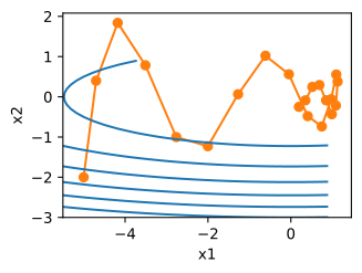

epoch 20, x1: 0.195696, x2: -0.249649

The iterate orbits the minimum before settling. Over-damped ↔︎ crawl; under-damped ↔︎ ringing; \beta^\star = critical damping.

From scratch

Velocity = one buffer per parameter, carried in states:

def init_momentum_states(feature_dim):
    v_w = d2l.zeros((feature_dim, 1))
    v_b = d2l.zeros(1)
    return [v_w, v_b]

def sgd_momentum(params, grads, states, hyperparams):
    for i in range(len(params)):
        states[i] = hyperparams['momentum'] * states[i] + grads[i]
        params[i] = params[i] - hyperparams['lr'] * states[i]
    return params[0], params[1]

On the airfoil harness

\beta = 0.5, \eta = 0.02:

def train_momentum(lr, momentum, num_epochs=2):
    d2l.train_ch11(sgd_momentum, init_momentum_states(feature_dim),
                   {'lr': lr, 'momentum': momentum}, data_iter,
                   feature_dim, num_epochs)

data_iter, feature_dim = d2l.get_data_ch11(batch_size=10)
train_momentum(0.02, 0.5)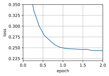

loss: 0.242, 1.116 sec/epoch

\beta = 0.9 quintuples the effective step \eta/(1-\beta) — so lower \eta to 0.01, then 0.005:

train_momentum(0.01, 0.9)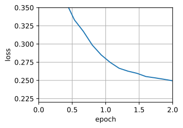

loss: 0.251, 0.332 sec/epoch

train_momentum(0.005, 0.9)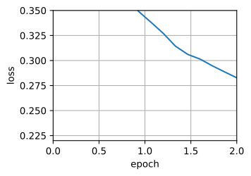

loss: 0.245, 0.324 sec/epoch

Concise: one argument

trainer = optax.sgd
d2l.train_concise_ch11(trainer, {'learning_rate': 0.005, 'momentum': 0.9},
                       data_iter)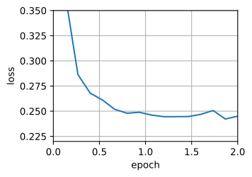

loss: 0.249, 0.352 sec/epoch

Nesterov: look before you leap

Evaluate the gradient at the point the velocity is taking you to:

\mathbf{v}_t = \beta \mathbf{v}_{t-1} + \nabla f(\mathbf{x}_{t-1} - \eta \beta \mathbf{v}_{t-1}),\qquad \mathbf{x}_t = \mathbf{x}_{t-1} - \eta \mathbf{v}_t.

About to overshoot? The look-ahead gradient already points back.

def nesterov_2d(x1, x2, v1, v2, f_grad):
    g1, g2 = f_grad(x1 - eta * beta * v1,  # Gradient at the look-ahead
                    x2 - eta * beta * v2)  # point, not at (x1, x2)
    v1, v2 = beta * v1 + g1, beta * v2 + g2
    return x1 - eta * v1, x2 - eta * v2, v1, v2

eta, beta = 0.3, 0.8
d2l.show_trace_2d(f_2d, d2l.train_2d(nesterov_2d, f_grad=f_2d_grad))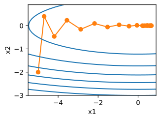

epoch 20, x1: 0.217791, x2: -0.000070

Same \eta, \beta as the ringing demo — oscillation gone.

Nesterov in practice

One flag; no extra gradient evaluations:

d2l.train_concise_ch11(
    optax.sgd,
    {'learning_rate': 0.005, 'momentum': 0.9, 'nesterov': True}, data_iter)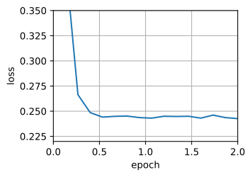

loss: 0.243, 0.343 sec/epoch

Guarantees heavy ball lacks: \mathcal{O}(1/k^2) convex (optimal), \sqrt{\kappa} beyond quadratics.
Small-batch noise dwarfs the correction → curves match plain momentum here. Matters when curvature dominates: large batches, \beta \to 1.

Recap

\mathbf{v}_t = \beta \mathbf{v}_{t-1} + \mathbf{g}_t, \mathbf{x}_t = \mathbf{x}_{t-1} - \eta \mathbf{v}_t.
Persistent components accumulate, oscillating ones cancel; noise smooths too.
\beta = timescale (\tfrac{1}{1-\beta} steps) and damping knob; tuned momentum: \kappa \to \sqrt{\kappa}.
Nesterov look-ahead: damps ringing, adds guarantees, costs nothing.
\beta = 0.9 is the default; Adam (:numref:sec_adam) keeps the idea and adds per-coordinate scaling.