class SquareRootScheduler:
    def __init__(self, lr=0.1):
        self.lr = lr

    def __call__(self, epoch):
        return self.lr * pow(epoch + 1.0, -0.5)

scheduler = SquareRootScheduler(lr=0.3)
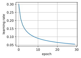
d2l.plot(d2l.arange(num_epochs), [scheduler(t) for t in range(num_epochs)],
xlabel='epoch', ylabel='learning rate')Baseline: constant \eta = 0.3
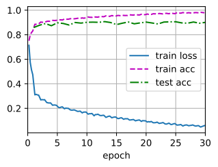
train loss 0.058, train acc 0.979, test acc 0.897Both failure modes on one plot: loss noisy to the end (riding the noise floor), and test accuracy stalls while train accuracy climbs — overfitting.
Square-root decay
\eta_t = \eta_0 (t+1)^{-1/2} — the convex-optimal rate from 9.3. A scheduler is a callable:
Square-root decay: training
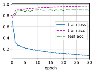
train loss 0.085, train acc 0.971, test acc 0.905The loss is smoother, but test accuracy remains below the constant baseline. The rate is too small at both ends: gives up the high early rate within ~3 epochs, yet ends with the largest tail \eta of any decay here. Shape matters.
Multiplicative and piecewise constant
\eta_t = \max(\eta_{\min}, \eta_0\, \alpha^t) — aggressive, floor as safety net:
class FactorScheduler:
    def __init__(self, factor=1, stop_factor_lr=1e-7, base_lr=0.1):
        self.factor = factor
        self.stop_factor_lr = stop_factor_lr
        self.base_lr = base_lr

    def __call__(self, epoch):
        return max(self.stop_factor_lr, self.base_lr * self.factor ** epoch)

scheduler = FactorScheduler(factor=0.9, stop_factor_lr=0.01, base_lr=0.3)
d2l.plot(d2l.arange(50), [scheduler(t) for t in range(50)],
         xlabel='epoch', ylabel='learning rate')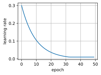
Piecewise constant decay reduces the rate after progress stalls at each noise floor, producing the ImageNet-era staircase:
class MultiFactorScheduler:
    def __init__(self, milestones, factor, base_lr):
        self.milestones = milestones
        self.factor = factor
        self.base_lr = base_lr

    def __call__(self, epoch):
        lr = self.base_lr
        for milestone in self.milestones:
            if epoch >= milestone:
                lr *= self.factor
        return lr

scheduler = MultiFactorScheduler(milestones=[15, 25], factor=0.5, base_lr=0.3)
d2l.plot(d2l.arange(num_epochs), [scheduler(t) for t in range(num_epochs)],
         xlabel='epoch', ylabel='learning rate')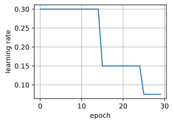
Cosine decay
\eta_t = \eta_T + \frac{\eta_0 - \eta_T}{2}(1 + \cos(\pi t / T))
One parameter, no milestones, no kinks (Loshchilov & Hutter, 2016).
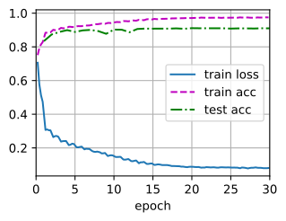
train loss 0.084, train acc 0.972, test acc 0.911The stay-high, decay-hard shapes (multiplicative, piecewise, cosine) beat the baseline and are too close to call from single runs. Cosine won on convenience, not measured superiority.
Warmup and initial stability
Even a BatchNorm network has a stability limit. A cold start at \eta = 7.5 (25× the baseline) remains at chance accuracy after one epoch:
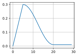
train loss 2.253, train acc 0.125, test acc 0.100A five-epoch ramp to the same rate permits training to reach 80–90% accuracy:
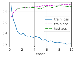
train loss 0.213, train acc 0.918, test acc 0.896Warmup + cosine
The default recipe of the late 2010s, and still strong:
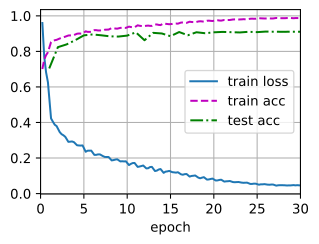
train loss 0.042, train acc 0.989, test acc 0.913Dependence of cosine decay on the horizon
The horizon T is baked in from step one.
- Mid-run checkpoints: rate never came down → not finished models.
- Want 2× the budget after the fact? Retrain.
- Scaling-law study at 5 budgets? 5 full runs.
Warmup–stable–decay (MiniCPM; Hu et al., 2024): warm up, hold the peak constant for most of the run, decay in the last 10–20%. Every plateau checkpoint is horizon-free; the decay is a harvest step.
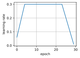
Loss reduction during WSD decay
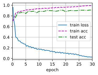
train loss 0.027, train acc 0.994, test acc 0.912Plateau loss remains above cosine’s, then decreases rapidly when the decay begins. Same final range as cosine at the same budget.
Branching off the plateau
Train warmup + stable only (no horizon committed), keep going as long as you like, then clone and decay whenever you want a finished model:
model_branch = nnx.clone(model_plateau)
decay = WSDScheduler(max_update=6, decay_steps=6, base_lr=0.3, final_lr=0.01)
train(model_branch, train_iter, test_iter, 6, lr, decay, animator=board,
      epoch_offset=30)
board.fig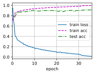
train loss 0.015, train acc 0.998, test acc 0.905The branch reaches the accuracy range of the full cosine run even though the horizon is chosen afterward. One plateau run can therefore supply branched decays for several budgets (Hägele et al., 2024).
Plain SGD carries no state, so cloning parameters sufficed. With momentum or Adam, branch the optimizer state too.