Adagrad

Adaptive Learning Rates

What if different parameters need different learning rates? A rare feature gets updated once per million steps; a common one every step. Sharing \eta forces a compromise — too small for the rare, too large for the common.

Adagrad

Adagrad (Duchi, Hazan, Singer 2011) gives each parameter its own learning rate, scaled by the square root of all past squared gradients:

\mathbf{s}_t = \mathbf{s}_{t-1} + \mathbf{g}_t^2,\quad \mathbf{x}_t = \mathbf{x}_{t-1} - \frac{\eta}{\sqrt{\mathbf{s}_t + \epsilon}} \odot \mathbf{g}_t.

Coordinates with large gradients shrink their effective step; rarely-updated coordinates keep theirs. The seed of every modern adaptive optimizer.

Setup and demo

Same anisotropic quadratic. Adagrad self-adapts the step sizes per coordinate:

%matplotlib inline
from d2l import jax as d2l
import jax
from jax import numpy as jnp
import math
import numpy as np

Bigger learning rate is now safe — the \sqrt{\mathbf{s}_t} divisor handles the dynamic range:

def adagrad_2d(x1, x2, s1, s2):
    eps = 1e-6
    g1, g2 = 0.2 * x1, 4 * x2
    s1 += g1 ** 2
    s2 += g2 ** 2
    x1 -= eta / math.sqrt(s1 + eps) * g1
    x2 -= eta / math.sqrt(s2 + eps) * g2
    return x1, x2, s1, s2

def f_2d(x1, x2):
    return 0.1 * x1 ** 2 + 2 * x2 ** 2

eta = 0.4
d2l.show_trace_2d(f_2d, d2l.train_2d(adagrad_2d))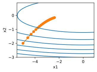

epoch 20, x1: -2.382563, x2: -0.158591

eta = 2
d2l.show_trace_2d(f_2d, d2l.train_2d(adagrad_2d))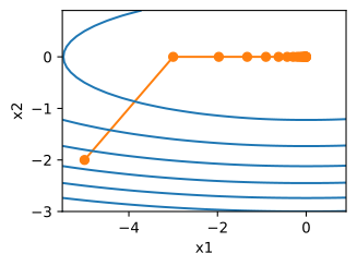

epoch 20, x1: -0.002295, x2: -0.000000

From-scratch Adagrad

Carry one accumulator \mathbf{s} per parameter. Add \epsilon to avoid division by zero on the first step:

def init_adagrad_states(feature_dim):
    s_w = jnp.zeros((feature_dim, 1))
    s_b = jnp.zeros(1)
    return [s_w, s_b]

def adagrad(params, grads, states, hyperparams):
    eps = 1e-6
    for i, (p, s, g) in enumerate(zip(params, states, grads)):
        s = s + jnp.square(g)
        params[i] = p - hyperparams['lr'] * g / jnp.sqrt(s + eps)
        states[i] = s
    return params[0], params[1]

data_iter, feature_dim = d2l.get_data_ch11(batch_size=10)
d2l.train_ch11(adagrad, init_adagrad_states(feature_dim),
               {'lr': 0.1}, data_iter, feature_dim);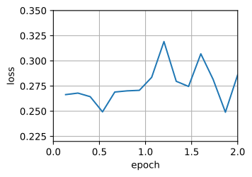

loss: 0.288, 1.134 sec/epoch

Concise: framework Adagrad

import optax
trainer = optax.adagrad
d2l.train_concise_ch11(trainer, {'learning_rate': 0.1}, data_iter)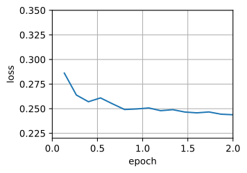

loss: 0.244, 0.716 sec/epoch

Recap

• Per-parameter learning rate, scaled by 1/\sqrt{\sum_t g_t^2}.
• Wins on sparse features — frequent ones cool down, rare ones keep moving.
• Failure mode: \mathbf{s}_t accumulates forever, so the effective \eta decays to zero — bad for non-convex problems where you keep needing updates. RMSProp fixes this by using an exponentially decaying \mathbf{s}_t instead.