Sentiment Analysis: Using Recurrent Neural Networks

Sentiment RNN

Sentiment classification on IMDb: pretrained word vectors → bidirectional LSTM → linear head. Standard pre-Transformer text-classification recipe.

The encoder reads the review left-to-right and right-to-left; concatenated final hidden states feed a binary classifier. GloVe gives a strong initialization that the LSTM then specializes for sentiment.

Pipeline

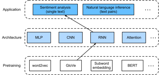
GloVe embeddings → BiLSTM → output classifier.

Setup

from d2l import jax as d2l
import jax
from jax import numpy as jnp
from flax import nnx
import optax
import numpy as np

batch_size = 128
train_iter, test_iter, vocab = d2l.load_data_imdb(batch_size)

BiRNN classifier

Class definition: embedding -> bidirectional LSTM -> concatenate the first and last hidden states -> 2-way decoder. The decoder input has width 4h: two directions times two endpoint states.

class BiRNN(nnx.Module):
    def __init__(self, vocab_size, embed_size, num_hiddens, num_layers,
                 rngs=None):
        rngs = nnx.Rngs(params=0, carry=1) if rngs is None else rngs
        self.embedding = nnx.Embed(vocab_size, embed_size, rngs=rngs)
        self.forward_rnns = nnx.List([])
        self.backward_rnns = nnx.List([])
        for i in range(num_layers):
            num_inputs = embed_size if i == 0 else 2 * num_hiddens
            self.forward_rnns.append(nnx.RNN(
                nnx.LSTMCell(num_inputs, num_hiddens, rngs=rngs), rngs=rngs))
            self.backward_rnns.append(nnx.RNN(
                nnx.LSTMCell(num_inputs, num_hiddens, rngs=rngs),
                reverse=True, keep_order=True, rngs=rngs))
        self.decoder = nnx.Linear(4 * num_hiddens, 2, rngs=rngs)

    def __call__(self, inputs):
        # The shape of `inputs` is (batch size, no. of time steps)
        embeddings = self.embedding(inputs)
        outputs = embeddings
        for forward_rnn, backward_rnn in zip(
                self.forward_rnns, self.backward_rnns):
            outputs = jnp.concatenate(
                [forward_rnn(outputs), backward_rnn(outputs)], axis=-1)
        # Each endpoint contains both directions, so concatenating the first
        # and last time steps produces 4 * num_hiddens features.
        encoding = jnp.concatenate([outputs[:, 0, :], outputs[:, -1, :]],
                                   axis=1)
        outs = self.decoder(encoding)
        return outs

BiRNN instance

Instantiate a 2-layer BiLSTM with 100-dimensional embeddings and 100 hidden units. Frameworks initialize recurrent weights differently, but the model contract is the same:

embed_size, num_hiddens, num_layers, devices = 100, 100, 2, d2l.try_all_gpus()
net = BiRNN(len(vocab), embed_size, num_hiddens, num_layers)

# NNX modules create their parameters in the constructor.
d2l.check_shape(net(jnp.ones((1, 500), dtype=jnp.int32)), (1, 2))

Loading pretrained GloVe

Use 100-dim GloVe vectors trained on Wikipedia + Gigaword. Initialize the embedding layer from them; freeze or fine-tune (we freeze — we do not update the pretrained GloVe vectors):

glove_embedding = d2l.TokenEmbedding('glove.6b.100d')

embeds = glove_embedding[vocab.idx_to_token]
embeds.shape

(49346, 100)

# Store the pretrained table as non-trainable NNX data.
net.embedding.embedding = nnx.data(jnp.array(embeds))

Training

Standard cross-entropy + Adam. Watch validation accuracy, not just training loss; sentiment models overfit quickly on IMDb if the embedding and classifier are too large:

lr, num_epochs = 0.01, 4
optimizer = nnx.Optimizer(net, optax.adam(lr), wrt=nnx.Param)
loss_fn = optax.softmax_cross_entropy_with_integer_labels

@nnx.jit
def train_step(net, optimizer, X, y):
    def compute_loss(model):
        logits = model(X)
        return loss_fn(logits, y).mean(), logits
    (loss, logits), grads = nnx.value_and_grad(
        compute_loss, has_aux=True)(net)
    optimizer.update(net, grads)
    return loss, logits

@nnx.jit
def eval_step(net, X):
    return net(X)

for epoch in range(num_epochs):
    loss_terms, train_correct_terms, num_train = [], [], 0
    for X, y in train_iter:
        l, logits = train_step(net, optimizer, X, y)
        loss_terms.append(l * len(y))
        train_correct_terms.append((logits.argmax(axis=-1) == y).sum())
        num_train += len(y)
    # Evaluate
    correct_terms, total = [], 0
    for X, y in test_iter:
        logits = eval_step(net, X)
        correct_terms.append((logits.argmax(axis=-1) == y).sum())
        total += len(y)
    loss_sum = float(jnp.stack(loss_terms).sum())
    train_correct = int(jnp.stack(train_correct_terms).sum())
    correct = int(jnp.stack(correct_terms).sum())
    print(f'epoch {epoch + 1}, loss {loss_sum / num_train:.3f}, '
          f'train acc {train_correct / num_train:.3f}, '
          f'test acc {correct / total:.3f}')

epoch 1, loss 0.627, train acc 0.632, test acc 0.796
epoch 2, loss 0.418, train acc 0.814, test acc 0.825
epoch 3, loss 0.364, train acc 0.844, test acc 0.847
epoch 4, loss 0.333, train acc 0.857, test acc 0.846

def predict_sentiment(net, vocab, sequence):
    """Predict the sentiment of a text sequence."""
    sequence = jnp.array(vocab[sequence.split()])
    label = jnp.argmax(net(sequence.reshape(1, -1)), axis=1)
    return 'positive' if label == 1 else 'negative'

Predict on new reviews

The final check should classify clearly positive and clearly negative synthetic reviews differently. This is not a full evaluation, but it catches label/order mistakes in the pipeline.

predict_sentiment(net, vocab, 'this movie is so great')

'positive'

predict_sentiment(net, vocab, 'this movie is so bad')

'negative'

Recap

• BiLSTM-on-GloVe: a strong pre-Transformer baseline for text classification.
• Pretrained embeddings carry general-purpose word semantics; LSTM specializes for sentiment.
• Easily beaten today by fine-tuned BERT, but a clean template for sequence-to-label tasks more broadly.