Sentiment Analysis: Using Convolutional Neural Networks

textCNN

textCNN (Kim, 2014) — a 1D conv net for sentiment. Different architecture, same task as the RNN deck.

Why CNNs on text? Each filter is a learned n-gram detector. Run several filter widths in parallel (3, 4, 5 words) for multi-scale coverage. Max-over-time pool collapses position; concat → linear → softmax. Fast, strong, parallelizable.

Pipeline

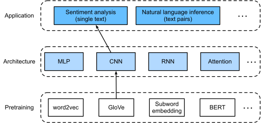
GloVe → 1D conv filters of varying widths → max-pool → classifier.

Setup

from d2l import jax as d2l
import jax
from jax import numpy as jnp
from flax import nnx
import optax
import numpy as np

batch_size = 256
train_iter, test_iter, vocab = d2l.load_data_imdb(batch_size)

1D convolution

Sliding kernel over a 1D sequence. Output element = elementwise multiply + sum of an n-token window:

1D conv: kernel (1, 2) slides over input; first output is 0 \cdot 1 + 1 \cdot 2 = 2.

def corr1d(X, K):
    w = K.shape[0]
    Y = d2l.zeros((X.shape[0] - w + 1))
    for i in range(Y.shape[0]):
        Y = Y.at[i].set((X[i: i + w] * K).sum())
    return Y

Multi-channel 1D conv

Embedding dim = input channels. Kernel has the same channel count; output is single-channel (or multi if you have multiple kernels).

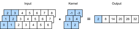
3-channel 1D conv.

X, K = d2l.tensor([0, 1, 2, 3, 4, 5, 6]), d2l.tensor([1, 2])
corr1d(X, K)

Array([ 2.,  5.,  8., 11., 14., 17.], dtype=float32)

Equivalent 2D-conv view

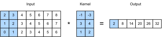
Equivalent to a 2D conv with kernel height = input height:

def corr1d_multi_in(X, K):
    # First, iterate through the 0th dimension (channel dimension) of `X` and
    # `K`. Then, add them together
    return sum(corr1d(x, k) for x, k in zip(X, K))

X = d2l.tensor([[0, 1, 2, 3, 4, 5, 6],
              [1, 2, 3, 4, 5, 6, 7],
              [2, 3, 4, 5, 6, 7, 8]])
K = d2l.tensor([[1, 2], [3, 4], [-1, -3]])
corr1d_multi_in(X, K)

Array([ 2.,  8., 14., 20., 26., 32.], dtype=float32)

Max-over-time pooling

Take the max over the time axis for each filter. Resulting feature is independent of where in the sequence the n-gram appeared. One scalar per filter, regardless of sentence length:

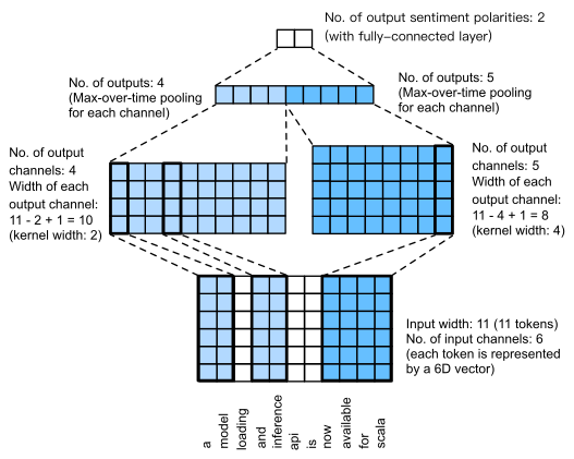
Max-over-time = max along the sequence axis.

textCNN model

Embedding (frozen GloVe + a fine-tunable copy) → parallel 1D convs at widths 3, 4, 5 → max-over-time → concat → dropout → linear:

class TextCNN(nnx.Module):
    def __init__(self, vocab_size, embed_size, kernel_sizes, num_channels,
                 rngs=None):
        rngs = nnx.Rngs(params=0, dropout=1) if rngs is None else rngs
        self.embedding = nnx.Embed(vocab_size, embed_size, rngs=rngs)
        # The embedding layer not to be trained
        self.constant_embedding = nnx.Embed(vocab_size, embed_size, rngs=rngs)
        self.dropout = nnx.Dropout(0.5, rngs=rngs)
        self.decoder = nnx.Linear(sum(num_channels), 2, rngs=rngs)
        # Create multiple one-dimensional convolutional layers
        self.convs = nnx.List([
            nnx.Conv(2 * embed_size, c, kernel_size=(k,), rngs=rngs)
            for c, k in zip(num_channels, kernel_sizes)])

    def __call__(self, inputs):
        # Concatenate two embedding layer outputs with shape (batch size, no.
        # of tokens, token vector dimension) along vectors
        embeddings = jnp.concatenate((
            self.embedding(inputs), self.constant_embedding(inputs)), axis=2)
        # For Flax Conv, input shape is (batch, length, channels) which is
        # already the shape of embeddings
        # For each one-dimensional convolutional layer, after max-over-time
        # pooling, a tensor of shape (batch size, no. of channels) is obtained.
        # Concatenate along channels
        encoding = jnp.concatenate([
            jnp.max(nnx.relu(conv(embeddings)), axis=1)
            for conv in self.convs], axis=1)
        outputs = self.decoder(self.dropout(encoding))
        return outputs

textCNN instance

The concrete model uses 100 channels at each kernel width. After max-over-time pooling, the classifier sees sum(num_channels) features, independent of review length.

embed_size, kernel_sizes, nums_channels = 100, [3, 4, 5], [100, 100, 100]
devices = d2l.try_all_gpus()
net = TextCNN(len(vocab), embed_size, kernel_sizes, nums_channels)
d2l.check_shape(nnx.view(net, deterministic=True)(
    jnp.ones((1, 500), dtype=jnp.int32)), (1, 2))

Loading pretrained GloVe

Both embedding tables start from the same GloVe vectors: one stays fixed as a semantic anchor, the other is fine-tuned for sentiment-specific cues.

glove_embedding = d2l.TokenEmbedding('glove.6b.100d')
embeds = glove_embedding[vocab.idx_to_token]
# Set pretrained embedding weights in the parameters
net.embedding.embedding[...] = jnp.array(embeds)
net.constant_embedding.embedding = nnx.data(jnp.array(embeds))

Training

CNNs train fast because all windows are processed in parallel. Use the metric output to compare with the BiLSTM deck: similar accuracy, less sequential computation.

lr, num_epochs = 0.001, 5
optimizer = nnx.Optimizer(net, optax.adam(lr), wrt=nnx.Param)
loss_fn = optax.softmax_cross_entropy_with_integer_labels

@nnx.jit
def train_step(net, optimizer, X, y):
    def compute_loss(model):
        logits = model(X)
        return loss_fn(logits, y).mean(), logits
    (loss, logits), grads = nnx.value_and_grad(
        compute_loss, has_aux=True)(net)
    optimizer.update(net, grads)
    return loss, logits

for epoch in range(num_epochs):
    loss_sum, train_correct, num_train = (
        jnp.array(0.0), jnp.array(0), 0)
    for X, y in train_iter:
        l, logits = train_step(net, optimizer, X, y)
        loss_sum += l * len(y)
        train_correct += (logits.argmax(axis=-1) == y).sum()
        num_train += len(y)
    # Evaluate
    correct, total = jnp.array(0), 0
    for X, y in test_iter:
        logits = nnx.view(net, deterministic=True)(X)
        correct += (logits.argmax(axis=-1) == y).sum()
        total += len(y)
    loss_sum, train_correct, correct = (
        float(loss_sum), int(train_correct), int(correct))
    print(f'epoch {epoch + 1}, loss {loss_sum / num_train:.3f}, '
          f'train acc {train_correct / num_train:.3f}, '
          f'test acc {correct / total:.3f}')

epoch 1, loss 0.644, train acc 0.664, test acc 0.812
epoch 2, loss 0.413, train acc 0.811, test acc 0.842
epoch 3, loss 0.339, train acc 0.851, test acc 0.856
epoch 4, loss 0.280, train acc 0.886, test acc 0.866
epoch 5, loss 0.219, train acc 0.916, test acc 0.875

tokens = jnp.array(vocab['this movie is so great'.split()])
logits = nnx.view(net, deterministic=True)(tokens.reshape(1, -1))
'positive' if int(jnp.argmax(logits, axis=1)[0]) == 1 else 'negative'

'positive'

tokens = jnp.array(vocab['this movie is so bad'.split()])
logits = nnx.view(net, deterministic=True)(tokens.reshape(1, -1))
'positive' if int(jnp.argmax(logits, axis=1)[0]) == 1 else 'negative'

'negative'

Recap

• textCNN = parallel 1D convs over word embeddings + max pooling + linear head.
• Each filter learns an n-gram detector; different widths give multi-scale coverage.
• Comparable accuracy to BiLSTM on IMDb at a fraction of the training time and zero recurrence.
• The shape (parallel filter widths, pooled features) is the template for many text-classification CNNs that followed.