Predicting House Prices on Kaggle

Dive into Deep Learning · §4.7

Predicting house prices on Kaggle
An end-to-end pipeline: messy data in, a scored prediction out. The difference between an underfit baseline and a converged one is nothing but training it properly.

The model is five lines; the pipeline is the lesson

Motivation

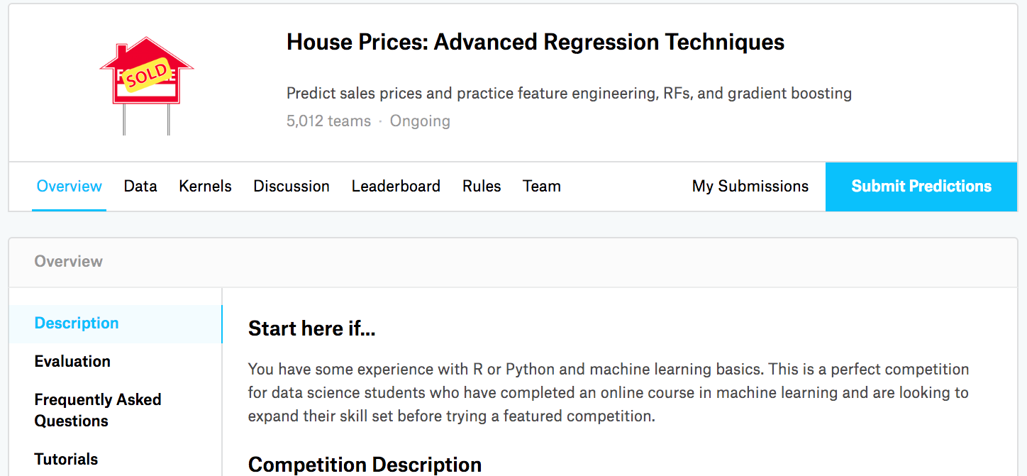
The Ames, Iowa housing competition: 1460 labelled houses, 80 mixed features, predict the sale price of 1459 more.

raw data is heterogeneous (numbers and categories) and has missing values;
prices span 10×, so the wrong loss over-weights mansions;
only ~1500 rows, so one train/val split is noisy.

Preprocess, match the loss to the metric, cross-validate, submit. That recipe outlives any single model.

Everything here works for any model class, not just neural nets.

The competition

what Kaggle is, and what this dataset asks

Kaggle in 30 seconds

The competition

Kaggle hosts open ML competitions. Download the train and test CSVs, train locally, upload predictions, get scored on a held-out slice of the test set.

A public/private split on the test labels stops competitors from overfitting the leaderboard.

The Kaggle competition platform: pick a competition, grab the data, submit predictions.

The House Prices competition page

The competition

The data is generic on purpose: no images, audio, or sequences, just a spreadsheet of house attributes and one price column.

That makes it the perfect first capstone, the whole job is the pipeline around the model.

The “Data” tab holds the train/test CSVs; the leaderboard scores each submission instantly.

Reading & preprocessing

from a messy DataFrame to clean tensors

One imports cell, then read the CSVs

Setup

A single per-framework imports cell. We read the data with pandas and d2l.download, a reusable hash-checked cache we lean on throughout the book:

%matplotlib inline
from d2l import jax as d2l
import jax
from jax import numpy as jnp
import numpy as np
import pandas as pd

download verifies a file’s SHA-1 and reuses the cached copy, so re-running never re-fetches.

Wrap train and test in a DataModule

Reading the data

A KaggleHouse(d2l.DataModule) holds the raw train and test frames:

class KaggleHouse(d2l.DataModule):
    def __init__(self, batch_size, train=None, val=None):
        super().__init__()
        self.save_hyperparameters()
        if self.train is None:
            self.raw_train = pd.read_csv(d2l.download(
                d2l.DATA_URL + 'kaggle_house_pred_train.csv', self.root,
                sha1_hash='585e9cc93e70b39160e7921475f9bcd7d31219ce'))
            self.raw_val = pd.read_csv(d2l.download(
                d2l.DATA_URL + 'kaggle_house_pred_test.csv', self.root,
                sha1_hash='fa19780a7b011d9b009e8bff8e99922a8ee2eb90'))

Train carries the label column, test does not, and that is what we predict:

data = KaggleHouse(batch_size=64)
print(data.raw_train.shape)
print(data.raw_val.shape)

(1460, 81)
(1459, 80)

What a few rows look like

Reading the data

print(data.raw_train.iloc[:4, [0, 1, 2, 3, -3, -2, -1]])

   Id  MSSubClass MSZoning  LotFrontage SaleType SaleCondition  SalePrice
0   1          60       RL         65.0       WD        Normal     208500
1   2          20       RL         80.0       WD        Normal     181500
2   3          60       RL         68.0       WD        Normal     223500
3   4          70       RL         60.0       WD       Abnorml     140000

Numbers (LotFrontage), categories (MSZoning, SaleType), an Id that carries no signal, and the target SalePrice. Models eat tensors, not DataFrames, so preprocessing is mandatory.

Three transforms turn features into tensors

Preprocessing

Impute missing numbers with the column mean.
Standardize each numeric column to mean 0, variance 1, so wildly different scales become comparable.
One-hot encode every category; a missing category becomes its own column (missing-as-signal).

Fit the mean and std on train only, then apply them to test. Using test statistics is leakage and flatters every later score.

One method: impute, standardize, one-hot

Preprocessing

Fit means, standard deviations, and the categorical vocabulary on the training rows, then apply that state to held-out rows. During cross-validation, “training rows” means the K-1 folds, not the complete labeled dataset:

def preprocess(self):
    self.train, self.val = fit_preprocess(self.raw_train, self.raw_val)

def fit_preprocess(train_raw, other_raw):
    """Fit preprocessing on train_raw and apply it to both dataframes."""
    label = 'SalePrice'
    train_X = train_raw.drop(columns=['Id', label])
    other_X = other_raw.drop(columns=['Id', label], errors='ignore')
    numeric = train_X.select_dtypes(include='number').columns
    train_X[numeric] = train_X[numeric].astype(float)
    other_X[numeric] = other_X[numeric].astype(float)
    mean, std = train_X[numeric].mean(), train_X[numeric].std()
    std = std.mask(std == 0, 1)
    train_X.loc[:, numeric] = (train_X[numeric] - mean) / std
    other_X.loc[:, numeric] = (other_X[numeric] - mean) / std
    train_X.loc[:, numeric] = train_X[numeric].fillna(0)
    other_X.loc[:, numeric] = other_X[numeric].fillna(0)
    train_X = pd.get_dummies(train_X, dummy_na=True)
    other_X = pd.get_dummies(other_X, dummy_na=True)
    other_X = other_X.reindex(columns=train_X.columns, fill_value=0)
    train_X[label] = train_raw[label].values
    if label in other_raw:
        other_X[label] = other_raw[label].values
    return train_X, other_X

The right loss

match what you train to what you are scored on

Prices are relative, so score the logarithm

Error measure

A $100k miss on a $125k house is a disaster; on a $4M house it is a great prediction. We care about relative error, so predict \log(\text{price}) and score the root-mean-squared log error:

\textrm{RMSLE} = \sqrt{\frac{1}{n}\sum_{i=1}^{n}\big(\log y_i - \log \hat{y}_i\big)^2}.

This is the official Kaggle metric here. Errors are penalized as percentages, not dollars.

Loss in code

Error measure

The data loader hands back features and the log of the price, so an ordinary squared-error loss already trains against log-RMSE:

def get_dataloader(self, train):
    label = 'SalePrice'
    data = self.train if train else self.val
    if label not in data: return
    get_tensor = lambda x: d2l.tensor(x.values.astype(float),
                                      dtype=d2l.float32)
    # Logarithm of prices 
    tensors = (get_tensor(data.drop(columns=[label])),  # X
               d2l.reshape(d2l.log(get_tensor(data[label])), (-1, 1)))  # Y
    return self.get_tensorloader(tensors, train)

Taking the log in the loader means the model and loss code stay completely standard.

K-fold cross-validation

a stable score from a small dataset

K-fold cross-validation

Model selection

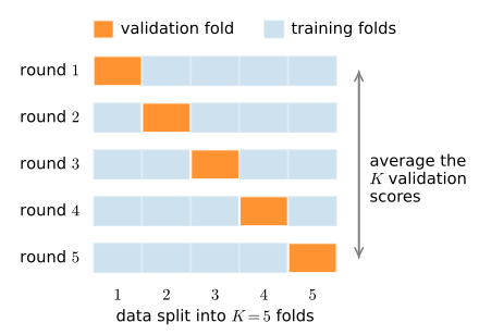
With ~1500 rows, one 80/20 split is noisy. Split the data into K folds; train K times, each time holding out a different fold; average the K validation scores.

Costs K\times the compute, buys a far steadier estimate, and the same loop supports hyperparameter search. Fit preprocessing anew inside each training fold; otherwise the held-out fold leaks into the model pipeline.

Each round holds out one fold for validation (orange) and trains on the other four (blue); the estimate is the mean of the five scores.

K-fold in code

Model selection

k_fold_data slices out fold i as validation and trains on the rest. Then fit a fresh model per fold and average the held-out scores; NNX models retain their trained parameters directly, so the same ensemble structure works across frameworks:

def k_fold(trainer, data, k, model_fn):
    val_loss, models = [], []
    for i, data_fold in enumerate(k_fold_data(data, k)):
        # One-hot vocabularies are fitted within each fold, so the number of
        # input columns can differ slightly between folds.
        model = model_fn(data_fold)
        model.board.yscale='log'
        if i != 0: model.board.display = False
        trainer.fit(model, data_fold)
        val_loss.append(float(model.board.data['val_loss'][-1].y))
        models.append((model, data_fold.test))
    print(f'average validation log mse = {sum(val_loss)/len(val_loss)}')
    return models

Model selection

a competent baseline, then a small MLP

A baseline only counts if trained to convergence

Model selection

Start with a linear model through the same K-fold loop, and train it competently: 100 epochs at learning rate 0.03, not the customary ten:

trainer = d2l.Trainer(max_epochs=100)
models = k_fold(
    trainer, data, k=5,
    model_fn=lambda fold: d2l.LinearRegression(
        fold.train.shape[1] - 1, lr=0.03))

Ten epochs of SGD leaves this model badly underfit; trained to convergence it reaches \approx 0.036. An underfit baseline flatters every model compared against it.

The verdict: the MLP edges ahead

Model selection

The natural next step is a small MLP: one 32-unit ReLU hidden layer, dropout 0.1, weight decay 10^{-4}; anything bigger overfits 1460 rows. Run through the same K-fold loop, learning rate, and epoch budget, it edges out the competently trained linear baseline: about 0.027 vs 0.036.

The lesson is deliberately undramatic: the nonlinearity buys only a modest gain here, and the bulk of the improvement over a careless, underfit baseline came from training either model to convergence. On small tabular data, gradient-boosted trees would still win.

Submit: ensemble the folds, write the CSV

Submitting

Average the K log-price predictions, exponentiate, submit:

preds = [model(d2l.tensor(test.values.astype(float), dtype=d2l.float32))
         for model, test in models]
# Average the K log-price predictions in log space, then exponentiate.
ensemble_preds = d2l.exp(d2l.reduce_mean(d2l.concat(preds, 1), 1))
submission = pd.DataFrame({'Id':data.raw_val.Id,
                           'SalePrice':d2l.numpy(ensemble_preds)})
submission.to_csv('submission.csv', index=False)

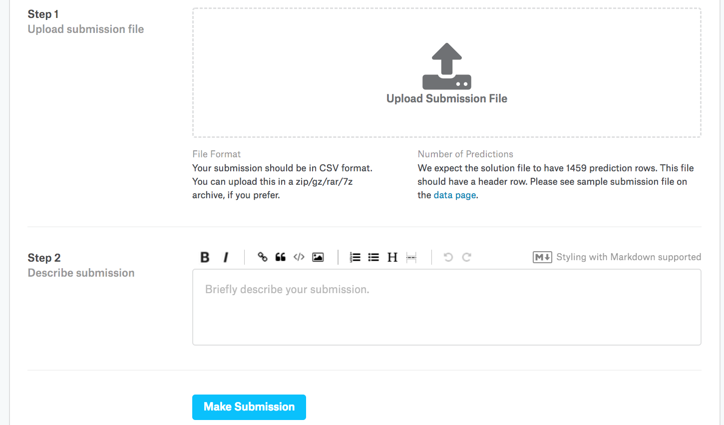
Upload the CSV and Kaggle scores it instantly.

The log-space mean averages predictions in the space where RMSLE measures error; exponentiating makes it a geometric mean in price space. This does not guarantee an improvement. The CV score measured a single fold model; refitting on all data is the more direct alternative to this fold ensembling.

The general competition recipe

Wrap-up

Download the train and test data.
Preprocess: impute, standardize, one-hot (all state fit on train).
Match the loss to the scoring metric.
K-fold CV for a generalization estimate and HP search.

Ensemble the fold models (log-space mean), or refit on all data with the chosen hyperparameters.
Submit in the host’s format.

Trees (XGBoost, LightGBM) usually win small tabular data; nets shine on images, text, audio. The pipeline is identical.

Recap

Wrap-up

Real ML is mostly pipeline, not architecture.
Heterogeneous data: impute, standardize, one-hot, with statistics fit on train only (no leakage).
Match the loss to the metric: log-RMSE for prices.

K-fold CV reduces split dependence on small IID data and drives HP search; fit preprocessing within every fold.
A baseline counts only if trained competently: underfit vs converged, same model.
Ensemble the folds in log space (or refit), then submit.
The model is a few lines; everything around it is the lesson.

That closes the MLP chapter. Next: the builder’s guide, covering layers, blocks, parameters, and custom architectures, the engineering that scales these ideas up.