Statistics

Dive into Deep Learning · §26.5

Estimators, hypothesis tests, and confidence intervals
statistics for practitioners.

Why statistics?

Motivation

A trained model is a guess made from random data. Statistics says how far that guess sits from the truth, whether an improvement is real, and how much to trust a number.

• Bias–variance = the under/overfit U-curve.
• p-values behind every A/B test and benchmark claim.
• Confidence intervals behind the error bars on a loss curve.

01

Estimators and their quality

bias, variance, MSE, consistency, efficiency

An estimator is a random variable

Estimators

\hat\theta_n = \hat f(x_1,\dots,x_n) is computed from a random sample, so it has a sampling distribution: it would land somewhere else on a fresh dataset.

That randomness is the whole subject: how much would the answer move, and is it centered on the truth?

Bias and variance

Estimators

\operatorname{Bias}(\hat\theta_n) = \mathbb E[\hat\theta_n] - \theta, \quad \operatorname{Var}(\hat\theta_n) = \mathbb E\bigl[(\hat\theta_n - \mathbb E[\hat\theta_n])^2\bigr].

Bias is a systematic offset (it does not wash out with more data); variance is measured against the estimator’s own center, not the truth.

Consistency and efficiency

Estimators

Consistent: \hat\theta_n\xrightarrow{P}\theta, guaranteed if both bias and variance vanish (the weak law of large numbers is the prototype).

Efficient: smallest variance among unbiased estimators. The Cramér–Rao bound is the floor; the MLE reaches it asymptotically.

MSE: one number for both errors

Estimators

\operatorname{MSE}(\hat\theta_n) = \mathbb E[(\hat\theta_n-\theta)^2] folds both errors into one number.

Proposition. \operatorname{MSE}(\hat\theta_n) = \operatorname{Bias}(\hat\theta_n)^2 + \operatorname{Var}(\hat\theta_n).

Proof: the cross term vanishes

Estimators

Let \mu=\mathbb E[\hat\theta_n] and split \hat\theta_n-\theta = (\hat\theta_n-\mu) + (\mu-\theta).

Squaring and taking expectations, the cross term is 2(\mu-\theta)\,\mathbb E[\hat\theta_n-\mu] = 0, leaving \operatorname{Var} + \operatorname{Bias}^2. \blacksquare

Markov then gives P(|\hat\theta_n-\theta|>\varepsilon)\le \operatorname{MSE}/\varepsilon^2: small MSE forces consistency, and for the sample mean this proves the weak law of large numbers.

Verify it in code

Estimators

Ten thousand sample means of n=30 Gaussian draws; the two sides of the decomposition agree to floating point:

import numpy as onp
theta_true, sigma = 1.0, 4.0
num_datasets, n = 10000, 30  # 10k datasets, each of n=30 points
samples = onp.random.normal(theta_true, sigma, (num_datasets, n))
theta_hats = samples.mean(axis=1)  # one sample-mean estimate per dataset

import numpy as onp
bias = stat_bias(theta_true, theta_hats)
# Default ddof=0: the plug-in variance of the estimates, which makes the
# identity exact for empirical averages (the n-1 variant is the next subsection)
var = onp.var(theta_hats)
mse(theta_hats, theta_true), var + onp.square(bias)

(np.float64(0.5404682200202031), np.float64(0.540468220020203))

The U-curve = generalization

Estimators

As model complexity grows, bias falls and variance rises; expected test error is their sum plus irreducible noise:

\text{err} = \operatorname{Bias}^2 + \operatorname{Var} + \sigma^2.

Regularization deliberately adds bias to cut variance more.

Why divide by n − 1?

Estimators

Deviations from \bar x are too small (it minimizes them), so dividing by n is biased low.

Proposition. s^2 = \tfrac{1}{n-1}\sum_i (x_i-\bar x)^2 has \mathbb E[s^2]=\sigma^2; one degree of freedom is spent estimating \bar x.

import numpy as onp
n = 3  # small n makes the 1/n bias glaring; the gap shrinks like 1/n
data = onp.random.normal(0, 2, (100000, n))  # sigma^2 = 4
dev2 = onp.square(data - data.mean(axis=1, keepdims=True)).sum(axis=1)
print('true variance    = 4')
print(f'E[divide by n]   = {float((dev2 / n).mean()):.3f}  (biased)')
print(f'E[divide by n-1] = {float((dev2 / (n - 1)).mean()):.3f}  (unbiased)')

true variance    = 4
E[divide by n]   = 2.676  (biased)
E[divide by n-1] = 4.013  (unbiased)

02

Hypothesis testing

null & alternative, test statistic, p-value, power

Two kinds of error

Testing

We never prove H_0, only reject it or fail to:

\alpha = P(\text{reject}\mid H_0), \qquad \beta = P(\text{fail}\mid H_A).

\alpha = significance (false positive); 1-\beta = power. For a composite H_A, \beta and the power are evaluated at a given alternative.

Significance and power

Testing

Fix \alpha (often 0.05) and target power (often 0.8). The sample size for the z-test to detect a standardized effect \delta (effect in units of noise) scales as n\propto 1/\delta^2.

A 0.01 improvement needs tens of thousands of test examples to confirm: why marginal benchmark gains are fragile.

A test in five steps

Testing

1. State H_0 and H_A.
2. Fix \alpha and a target power → required n.
3. Collect data.
4. Compute the statistic T(x) and its p-value.
5. Reject H_0 iff p\le\alpha.

A p-value is P(\text{data this extreme}\mid H_0), not P(H_0\mid\text{data}).

The rejection region

Testing

p = P_{H_0}\bigl(|T| \ge |t_{\text{obs}}|\bigr); land in the tails of total mass \alpha and reject.

Run m tests and P(\ge 1\text{ false win}) = 1-(1-\alpha)^m. Bonferroni tests at \alpha/m; at ML scale, control the false-discovery rate.

A worked test: two models

Testing

Is model B better, or is the gap noise? Under H_0 the labels are exchangeable: shuffle them, recompute the gap, repeat 10{,}000 times; the histogram is the null distribution, no Gaussian assumed:

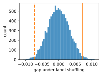
observed gap        = 0.0073
permutation p-value = 0.0197

The observed 0.73\% gap sits in the far tail: p\approx 0.02, real, but only just, with 20 seeds.

03

Quantifying uncertainty

confidence intervals and the bootstrap

What a confidence interval is

Intervals

A random interval C_n with P_\theta(C_n \ni \theta)\ge 1-\alpha for all \theta. The interval is random; \theta is fixed.

Correct reading: across many repetitions, 95\% of the constructed intervals trap \theta, not that this one does with probability 0.95 (that is a Bayesian credible interval, which needs a prior). Nothing about a single interval announces whether it trapped the truth.

The Gaussian interval

Intervals

For Gaussian data T=(\hat\mu_n-\mu)/(\hat\sigma_n/\sqrt n) is Student-t, near standard normal for large n (\hat\sigma_n\to\sigma plus Slutsky); the CLT extends the interval to non-Gaussian data:

\Bigl[\hat\mu_n - 1.96\,\tfrac{\hat\sigma_n}{\sqrt n},\; \hat\mu_n + 1.96\,\tfrac{\hat\sigma_n}{\sqrt n}\Bigr].

import numpy as onp
N = 1000
samples = onp.random.normal(loc=0, scale=1, size=(N,))
t_star = 1.96  # asymptotic value; small N would look this up in a t-table
mu_hat = onp.mean(samples)
se = samples.std(ddof=1) / onp.sqrt(N)  # ddof=1: unbiased sigma_hat
(mu_hat - t_star * se, mu_hat + t_star * se)

(np.float64(-0.08701890544137467), np.float64(0.036931924588281706))

Half-width shrinks like 1/\sqrt n: four times the data to halve the error bar.

Auditing the 95%

Intervals

“Roughly 95\% of the time” is the Neyman guarantee, and it is checkable: one thousand fresh datasets, one interval each, count the hits:

937 of 1000 intervals contain the true mean (expected about 950)

This run counts 937; the true target is \approx 947, not 950: at n=100 the exact t-quantile is a touch wider than 1.96. The count is the coverage picture rendered as a number, the only sense in which any interval is ever “95\% sure.”

Error bars propagate through functions

Intervals

Reporting g(\hat\theta) instead of \hat\theta? First-order Taylor says the fluctuation scales by the local slope, the delta method:

\operatorname{se}\bigl(g(\hat\theta)\bigr) \;\approx\; \bigl|g'(\hat\theta)\bigr|\;\operatorname{se}(\hat\theta).

Accuracy \hat p = 0.90 on n=1000 examples has \operatorname{se} \approx 0.0095; reported as log-odds, the slope 1/(\hat p(1-\hat p)) \approx 11.1 stretches the error bar to \approx 0.105.

A gradient replaces g' for vector parameters; when no derivative is convenient, the bootstrap (next) sidesteps the calculus entirely.

The bootstrap: many statistics, no formula

Intervals

Substitute the empirical distribution for the unknown one: resample n points with replacement, recompute the statistic, repeat.

Works for the median, AUC, accuracy, BLEU: anywhere no closed-form standard error exists.

Bootstrap in code

Intervals

The bootstrap SE and a percentile interval for a skewed sample’s median:

sample median        = 0.808
bootstrap SE         = 0.072
percentile 95% CI    = (0.682, 0.955)

The mean’s Gaussian interval lands elsewhere; same data, different statistic, different answer:

Gaussian 95% CI (mean) = (0.986, 1.272)

Recap

Wrap-up

• Estimators are random; quality = bias, variance, and their sum, MSE = \operatorname{Bias}^2+\operatorname{Var}.
• Consistent when both vanish; the U-curve is under/overfitting as one identity; n-1 pays for one degree of freedom.

• Testing: control \alpha, want power \ge 0.8; the p-value is data-given-null, not null-given-data; correct for multiplicity.
• Intervals often shrink like 1/\sqrt n; the bootstrap gives error bars for many regular statistics, with specialized resampling for dependent data.

The MSE split, the U-curve, and the CLT recur throughout the book.