Bayesian Computation

Dive into Deep Learning · §26.4

How to average over everything you don’t know
Bayesian computation.

Why keep the posterior?

Motivation

Optimization returns one \boldsymbol\theta; many others explain the data about as well, and they disagree about the next prediction. Averaging over them is the posterior predictive

p(y_\star\mid\mathbf x_\star,\mathcal D) =\int p(y_\star\mid\mathbf x_\star,\boldsymbol\theta)\, p(\boldsymbol\theta\mid\mathcal D)\,d\boldsymbol\theta.

• calibrated uncertainty instead of overconfident plug-in
• the integral has no closed form outside conjugate pairs

The whole subject: average over a distribution you can only evaluate, up to a constant.

01

The target

a nonconjugate posterior, and an exact reference to audit against

The smallest real problem

The target

Bayesian logistic regression: sigmoid likelihood, Gaussian prior — no conjugate rescue.

p(\boldsymbol\theta\mid\mathcal D)\propto \prod_i\sigma(\mathbf z_i^\top\boldsymbol\theta)^{y_i} (1-\sigma(\mathbf z_i^\top\boldsymbol\theta))^{1-y_i} \exp\!\left(-\tfrac{\|\boldsymbol\theta\|^2}{2\tau^2}\right).

Two operations stay cheap, and every method is built from them: evaluate \log\widetilde p (up to a constant), and its gradient.

A grid gives ground truth (here!)

The target

Two parameters \Rightarrow quadrature on a 241\times241 grid is exact enough to audit everything. In d dimensions it costs m^d — the curse that makes the rest of the lecture necessary.

b0 = np.linspace(-2.5, 1.5, 241)
b1 = np.linspace(0.0, 2.8, 241)
B0, B1 = np.meshgrid(b0, b1, indexing='ij')
grid_theta = np.stack([B0.ravel(), B1.ravel()], axis=1)
grid_logp = log_joint(grid_theta)
grid_weight = np.exp(grid_logp - grid_logp.max())
grid_weight /= grid_weight.sum()
posterior_mean = grid_weight @ grid_theta
centered = grid_theta - posterior_mean
posterior_cov = (centered * grid_weight[:, None]).T @ centered
print('grid posterior mean:', posterior_mean.round(4))
print('grid posterior sd  :', np.sqrt(np.diag(posterior_cov)).round(4))
print('grid correlation   :',
      round(posterior_cov[0, 1] /
            np.sqrt(posterior_cov[0, 0] * posterior_cov[1, 1]), 4))

grid posterior mean: [-0.3335  1.4794]
grid posterior sd  : [0.3353 0.2871]
grid correlation   : -0.2288

What averaging buys

The target

The posterior predictive is pulled toward \tfrac12 relative to the plug-in MAP: averaging a nonlinear sigmoid \ne sigmoid of the average. Parameter uncertainty is a confidence discount.

theta_map = np.zeros(2)
for _ in range(12):
    probs = sigmoid(Z_bayes @ theta_map)
    precision = (Z_bayes.T @ (Z_bayes * (probs * (1 - probs))[:, None])
                 + np.eye(2) / prior_var)
    theta_map += np.linalg.solve(precision, grad_log_joint(theta_map)[0])
probs = sigmoid(Z_bayes @ theta_map)
laplace_precision = (Z_bayes.T @
                     (Z_bayes * (probs * (1 - probs))[:, None])
                     + np.eye(2) / prior_var)
laplace_cov = np.linalg.inv(laplace_precision)
print('MAP                 :', theta_map.round(4))
print('posterior mean      :', posterior_mean.round(4))

x_new = np.array([-2.0, 0.0, 2.0])
Z_new = np.column_stack([np.ones(len(x_new)), x_new])
pred_grid = grid_weight @ sigmoid(grid_theta @ Z_new.T)
pred_map = sigmoid(Z_new @ theta_map)
for x0, pm, pp in zip(x_new, pred_map, pred_grid):
    print(f'x={x0:+.1f}: plug-in MAP={pm:.3f}, posterior predictive={pp:.3f}')

MAP                 : [-0.3134  1.4039]
posterior mean      : [-0.3335  1.4794]
x=-2.0: plug-in MAP=0.042, posterior predictive=0.044
x=+0.0: plug-in MAP=0.422, posterior predictive=0.420
x=+2.0: plug-in MAP=0.924, posterior predictive=0.923

02

Importance sampling

sample somewhere easy, reweight by right-over-wrong

Correcting a proposal

Importance sampling

Draw from a tractable q, weight each draw by w=\widetilde p/q; self-normalizing cancels the unknown evidence:

\mathbb E_p[h]= \frac{\mathbb E_q[w\,h]}{\mathbb E_q[w]}.

Coverage is everything — and the weight ESS 1/\sum_s\bar w_s^2 cannot see mass that was never sampled.

Prior vs. Laplace proposal

Importance sampling

A proposal aimed at the posterior (Laplace) extracts more information from 5,000 draws than the broad prior does from 20,000.

def gaussian_logpdf(samples, mean, cov):
    diff = samples - mean
    sign, logdet = np.linalg.slogdet(cov)
    precision = np.linalg.inv(cov)
    return -0.5 * (len(mean) * np.log(2 * np.pi) + logdet
                   + np.einsum('ni,ij,nj->n', diff, precision, diff))

def importance(proposal_mean, proposal_cov, n, seed):
    local_rng = np.random.default_rng(seed)
    samples = local_rng.multivariate_normal(proposal_mean, proposal_cov, n)
    logw = log_joint(samples) - gaussian_logpdf(
        samples, proposal_mean, proposal_cov)
    weight = np.exp(logw - logw.max())
    weight /= weight.sum()
    mean = weight @ samples
    predictive = weight @ sigmoid(samples @ Z_new.T)
    ess = 1.0 / (weight @ weight)
    return mean, predictive, ess, weight.max()

prior_is = importance(np.zeros(2), prior_var * np.eye(2), 20000, 2)
laplace_is = importance(theta_map, laplace_cov, 5000, 3)
for name, result, n in [('prior proposal', prior_is, 20000),
                        ('Laplace proposal', laplace_is, 5000)]:
    mean, pred, ess, max_weight = result
    print(f'{name:18s}: ESS={ess:7.1f}/{n}, max weight={max_weight:.4f}, '
          f'mean={mean.round(4)}')

prior proposal    : ESS=  681.1/20000, max weight=0.0029, mean=[-0.3415  1.4898]
Laplace proposal  : ESS= 4287.3/5000, max weight=0.0025, mean=[-0.3359  1.4772]

03

Markov chain Monte Carlo

walk so that time spent equals posterior mass

The Metropolis rule

MCMC

Propose a local move; accept uphill always, downhill with probability \widetilde p(\boldsymbol\theta')/\widetilde p(\boldsymbol\theta) — only ratios, so the normalizer cancels.

\alpha=\min\!\left(1, \frac{\widetilde p(\boldsymbol\theta')\,q(\boldsymbol\theta\mid\boldsymbol\theta')} {\widetilde p(\boldsymbol\theta)\,q(\boldsymbol\theta'\mid\boldsymbol\theta)}\right)

Calibrated downhill moves give detailed balance: no net flow, so the posterior is stationary. Rejected proposals repeat the state — that is the weighting.

Four chains, dispersed starts

MCMC

chain 1: acceptance rate=0.525
chain 2: acceptance rate=0.526
chain 3: acceptance rate=0.526
chain 4: acceptance rate=0.527

Mixing, not draw count

MCMC

Correlated draws carry less information. Traces show sticking; split \widehat R\approx1 says chains agree; autocorrelation ESS converts MN states into equivalent independent draws, and MCSE \approx sd/\sqrt{N_{\text{eff}}}.

def split_rhat(x):
    m, n, d = x.shape
    half = n // 2
    split = np.concatenate([x[:, :half], x[:, half:2 * half]], axis=0)
    within = split.var(axis=1, ddof=1).mean(axis=0)
    between = half * split.mean(axis=1).var(axis=0, ddof=1)
    variance = (half - 1) * within / half + between / half
    return np.sqrt(variance / within)

def autocorrelation(x):
    x = x - x.mean()
    n = len(x)
    spectrum = np.fft.rfft(x, n=2 * n)
    acov = np.fft.irfft(spectrum * np.conj(spectrum))[:n]
    return acov / acov[0]

def teaching_ess(x):
    m, n, d = x.shape
    result = []
    for j in range(d):
        rho = np.mean([autocorrelation(x[c, :, j]) for c in range(m)], axis=0)
        positive_pairs = 0.0
        for lag in range(1, n - 1, 2):
            pair = rho[lag] + rho[lag + 1]
            if pair < 0:
                break
            positive_pairs += pair
        result.append(m * n / (1 + 2 * positive_pairs))
    return np.asarray(result)

d2l.use_svg_display()
flat_chains = chains.reshape(-1, 2)
rhat = split_rhat(chains)
ess = teaching_ess(chains)
mcmc_mean = flat_chains.mean(axis=0)
mcmc_sd = flat_chains.std(axis=0, ddof=1)
print('split R-hat:', rhat.round(4))
print('ESS        :', ess.round(0).astype(int))
print('MCMC mean  :', mcmc_mean.round(4),
      '  grid mean:', posterior_mean.round(4))
print('MCSE       :', (mcmc_sd / np.sqrt(ess)).round(4))

fig, axes = d2l.plt.subplots(1, 2, figsize=(10, 3.2))
for c in range(len(chains)):
    axes[0].plot(chains[c, :600, 1], linewidth=0.8, alpha=0.8)
axes[0].set(xlabel='post-warmup iteration', ylabel=r'slope $\theta_1$',
            title='four chain traces')
for c in range(len(chains)):
    axes[1].plot(autocorrelation(chains[c, :, 1])[:80], alpha=0.8)
axes[1].axhline(0, color='black', linewidth=0.7)
axes[1].set(xlabel='lag', ylabel='autocorrelation', title='serial dependence')
d2l.plt.tight_layout()
d2l.plt.show()

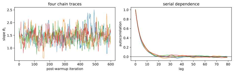
split R-hat: [1.0008 1.0004]
ESS        : [4521 4098]
MCMC mean  : [-0.3317  1.4768]   grid mean: [-0.3335  1.4794]
MCSE       : [0.005  0.0044]

04

Deterministic approximations

replace the posterior by the nearest tractable distribution

Laplace: the free Gaussian in every MAP

Laplace

At a maximum the linear Taylor term vanishes: locally the log posterior is a parabola, i.e. a Gaussian,

p(\boldsymbol\theta\mid\mathcal D)\approx \mathcal N(\boldsymbol\theta_{\text{MAP}},\,H^{-1}).

One Hessian beyond the optimization you were doing anyway. Local by construction: skew, tails, boundaries, other modes are invisible.

Variational inference: optimize a distribution

VI

Choose family q_\phi, maximize the ELBO — integration becomes optimization; reparameterize \boldsymbol\theta=\mathbf m+\mathbf s\odot\boldsymbol\epsilon and reuse Adam.

\mathcal L(\phi)=\mathbb E_{q_\phi}[\log p(\mathcal D,\boldsymbol\theta) -\log q_\phi(\boldsymbol\theta)]\le\log p(\mathcal D)

Reverse KL is mode-seeking: a too-simple family retreats into one mode and understates uncertainty. (This objective trains VAEs.)

All four methods, one posterior

Comparison

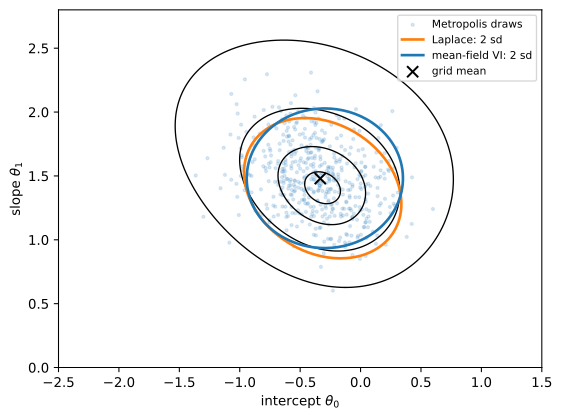
Exact contours; Metropolis draws trace them, skew included; Laplace is centered at the MAP; mean-field VI cannot tilt and is slightly narrow.

def covariance_ellipse(mean, cov, color, label):
    values, vectors = np.linalg.eigh(cov)
    angle = np.linspace(0, 2 * np.pi, 240)
    circle = np.stack([np.cos(angle), np.sin(angle)])
    ellipse = mean[:, None] + vectors @ (2 * np.sqrt(values)[:, None] * circle)
    d2l.plt.plot(ellipse[0], ellipse[1], color=color, linewidth=2, label=label)

d2l.plt.figure(figsize=(6, 4.5))
levels = np.quantile(grid_weight, [0.70, 0.90, 0.97, 0.995])
d2l.plt.contour(B0, B1, grid_weight.reshape(B0.shape),
                levels=np.unique(levels), colors='black', linewidths=1)
d2l.plt.scatter(flat_chains[::80, 0], flat_chains[::80, 1], s=5, alpha=0.15,
                label='Metropolis draws')
covariance_ellipse(theta_map, laplace_cov, 'tab:orange', 'Laplace: 2 sd')
covariance_ellipse(m_vi, vi_cov, 'tab:blue', 'mean-field VI: 2 sd')
d2l.plt.scatter(*posterior_mean, marker='x', s=70, color='black',
                label='grid mean')
d2l.plt.xlabel(r'intercept $\theta_0$')
d2l.plt.ylabel(r'slope $\theta_1$')
d2l.plt.legend(fontsize=8)
d2l.plt.tight_layout()
d2l.plt.show()

Takeaways

Summary

• Point estimates omit parameter uncertainty; the predictive integral is the Bayesian target, and all methods approximate it from \log\widetilde p and \nabla\log\widetilde p alone.
• Importance sampling: coverage first; ESS is blind to unseen mass.
• MCMC: time spent = posterior mass; judge by mixing, never by acceptance rate.
• Laplace: right peak, wrong tails, one Hessian. VI: optimization replaces integration; mode-seeking by construction.
• No scalar diagnostic proves an unseen mode does not exist.