Gradient-Based Optimization
Dive into Deep Learning · §26.1
Foundations of gradient-based optimization with -\nabla f
descent directions · smoothness · conditioning · momentum · stochastic gradients.
Foundations of gradient-based methods
Motivation
Before momentum, Adam, and learning-rate schedules, three questions have closed-form answers on quadratics:
- Why does a negative-gradient step make progress?
- How fast does it converge?
- What limits its rate?
Their answers depend on the condition number \kappa = \lambda_{\max}/\lambda_{\min}, read off the Hessian.
Develop the theory where it is exact (quadratics), then add momentum and noise to make it practical.
01
Directions & smoothness
where to step, and how far to trust it
Steepest descent is a theorem
Directions
A small step \eta\,\mathbf{d} changes f by \eta\,\nabla f^\top\mathbf{d} to first order, so \mathbf{d} is a descent direction when \nabla f^\top\mathbf{d} < 0. By Cauchy–Schwarz the steepest unit direction is unique:
\min_{\|\mathbf{d}\|=1}\nabla f^\top\mathbf{d} = -\|\nabla f\|, \qquad \mathbf{d}^\star = -\frac{\nabla f}{\|\nabla f\|}.
The local first-order model gives a half-space of descent directions. Each direction decreases the objective for sufficiently small positive steps; a finite step still needs smoothness or a line search.
Negative Directional Derivatives Give Descent
Directions
On f(x,y)=\tfrac12(x^2+10y^2): compare the first-order slope with the actual decrease, then scan 3600 directions for the most negative slope.
steepest -grad/|grad|:  slope = -10.1980,  f(x + eta d) - f(x) = -0.101498
diagonal -(1,1)/sqrt(2):  slope =  -8.4853,  f(x + eta d) - f(x) = -0.084578
axis     (-1,0):  slope =  -2.0000,  f(x + eta d) - f(x) = -0.019950
uphill   +(1,1)/sqrt(2):  slope =  +8.4853,  f(x + eta d) - f(x) = +0.085128
best of 3600 sampled unit directions: [-0.1959 -0.9806]  vs  -grad/|grad| = [-0.1961 -0.9806]
The brute-force winner lands on -\nabla f/\|\nabla f\|, to grid resolution.
Smoothness Bounds Finite Steps
Smoothness
The gradient changes along a finite step. Smoothness bounds that change: f is L-smooth when \|\nabla f(\mathbf{x})-\nabla f(\mathbf{y})\|\le L\|\mathbf{x}-\mathbf{y}\|, i.e. every Hessian eigenvalue lies in [-L,L]. This gives a quadratic upper bound and the descent lemma:
f(\mathbf{x}_{k+1}) \le f(\mathbf{x}_k) - \eta\big(1 - \tfrac{L\eta}{2}\big)\|\nabla f(\mathbf{x}_k)\|^2.
The first-order decrease \eta\|\nabla f\|^2 grows linearly; the curvature error \tfrac{L}{2}\eta^2\|\nabla f\|^2 grows quadratically. Progress for 0<\eta<2/L, best at \eta=1/L.
Smooth nonconvex objectives admit a stationarity bound
Smoothness
Telescoping the lemma at \eta=1/L, with f merely bounded below by f^\star:
\min_{0\le k<K}\|\nabla f(\mathbf{x}_k)\|^2 \;\le\; \frac{2L\,(f(\mathbf{x}_0)-f^\star)}{K}.
No convexity is needed. The result assumes global L-smoothness, a lower bound, and step 1/L. Under those assumptions it promises stationarity, not a minimum. Nonsmooth networks or trajectories without a useful smoothness bound fall outside the theorem.
Backtracking: a step near 1/L without knowing L
Smoothness
The local curvature varies, so no fixed step fits everywhere. Start optimistic and halve \eta until the Armijo sufficient-decrease condition holds, here on the quartic f(x)=\tfrac14 x^4:
fixed eta = 0.3 from x0 = 3:  |x_6| = 6.52e+103  (diverged)
accepted steps: [0.03125 0.0625  0.125   0.25    0.5     1.      1.      1.     ] ...
backtracking from x0 = 3:  f(x_25) = 1.09e-04  (monotone descent)
Fixed \eta=0.3 diverges from x_0=3; backtracking accepts 0.031, then increases as local curvature decreases. A line search estimates an acceptable step through objective evaluations.
02
The condition number
the quadratic model, solved exactly
Gradient descent decouples into modes
Quadratics
Near a minimum every smooth f is a quadratic \tfrac12\mathbf{x}^\top A\mathbf{x}. In the eigenbasis of A the iteration \mathbf{x}_{k+1}=(I-\eta A)\mathbf{x}_k splits into n independent geometric recursions, one per curvature eigenvalue:
c_i^{(k)} = (1-\eta\lambda_i)^k\,c_i^{(0)}.
- Stability needs |1-\eta\lambda_i|<1 for all modes: \eta<2/L.
- Speed is set by the slowest: \rho(\eta)=\max_i|1-\eta\lambda_i|.
The 2/L the descent lemma offered as sufficient is now necessary: past it the stiffest mode oscillates with growing amplitude.
Step-Size Regimes on a Quadratic
Quadratics
Sweep \eta across the ceiling on A=\mathrm{diag}(1,10), so L=10 and the ceiling is \eta=0.2:
 eta    |1-eta*1|  |1-eta*10|  spectral radius   |x_60|
0.020     0.980      0.800         0.980       3.0e-01
0.100     0.900      0.000         0.900       1.8e-03
0.182     0.818      0.818         0.818       8.3e-06
0.190     0.810      0.900         0.900       1.8e-03
0.200     0.800      1.000         1.000       1.0e+00
0.210     0.790      1.100         1.100       3.0e+02
Small \eta is stable but slow; \eta=2/11 balances the extreme modes and gives \rho=0.818; at \eta=0.2 the stiff mode alternates without contraction; above that threshold, its magnitude grows.
The Optimal Fixed Step on a Quadratic
Quadratics
Each step size draws a tent |1-\eta\lambda| with vertex at \lambda = 1/\eta; the rate is the taller endpoint over [\lambda_{\min}, \lambda_{\max}]. The best tent levels its endpoints:
\eta^\star = \frac{2}{\lambda_{\min}+\lambda_{\max}}, \qquad \rho(\eta^\star) = \frac{\kappa-1}{\kappa+1}.
Lowering either endpoint would raise the other.
With \eta^\star the iteration contracts by 0.818182, to six digits, at every step: on a quadratic the law is an exact identity.
Conditioning and Gradient-Descent Paths
Quadratics
The optimal step contracts by exactly (\kappa-1)/(\kappa+1), so the cost of gradient descent is linear in \kappa.
Stability chains the step to the steep mode while the flat mode barely moves: the zig-zag is the visible cost of a large \kappa.
Measured Edge-of-Stability Behavior
Quadratics
The classical advice: measure L, pick \eta < 2/L. Measured on a real (tiny) network, the causality runs backwards: same init, two step sizes, sharpness \lambda_{\max}(\nabla^2 f) tracked by finite differences:
        eta = 0.40 (2/eta = 5.0)   eta = 0.25 (2/eta = 8.0)
    k      loss    sharpness         loss    sharpness
     0    0.5097      3.32         0.5097      3.32
  4000    0.0124      4.94         0.0104      8.02
  8000    0.0008      4.97         0.0021      7.96
 12000    0.0007      5.00         0.0007      7.97
 16000    0.0005      5.00         0.0004      7.97
 20000    0.0004      5.00         0.0003      7.97
Training increases the measured sharpness toward 2/\eta (5.00 for \eta=0.4; within half a percent of 8 for \eta=0.25), then it remains near that value while the loss continues to decrease non-monotonically. The edge of stability: you pick \eta, the observed curvature depends on the selected step size.
Convexity upgrades stationarity to optimality
Quadratics
The \kappa-law generalizes from quadratics to convex functions. Each hypothesis upgrades what converges and how fast:
smooth only \;\min_k\|\nabla f\|^2 = O(1/k) (stationarity)
+ convex \;f-f^\star = O(1/k) (global values)
+ \mu-strongly convex \;f(\mathbf{x}_k)-f^\star \le (1-\tfrac{1}{\kappa})^k\,(f(\mathbf{x}_0)-f^\star)
linear, O(\kappa\log\tfrac1\varepsilon) steps
Stated here; proved with convexity in the next section.
03
Momentum, noise, curvature
making it practical at scale
Momentum is a damped oscillator
Acceleration
Give the iterate a velocity with memory, \mathbf{v}_{k+1}=\beta\mathbf{v}_k-\eta\nabla f. In each mode this is a mass-spring-damper and \beta is the damping knob: strong damping gives slow decay, weak damping gives oscillation, and critical tuning gives the fastest decay in this model.
Momentum Changes \kappa Dependence to \sqrt\kappa
Acceleration
Tuned heavy ball contracts every mode at (\sqrt{\kappa}-1)/(\sqrt{\kappa}+1); Nesterov’s look-ahead makes \sqrt{\kappa} a theorem beyond quadratics, and these rates are optimal for the stated first-order oracle classes. Compare all three at 10^{-6}:
kappa      GD   heavy ball   Nesterov     GD/kappa   HB/sqrt(kappa)
   10      69        27         43          6.9         8.5
  100     691        93        155          6.9         9.3
 1000    6908       315        508          6.9        10.0
GD’s count is linear in \kappa (6{,}908 at \kappa=1000); heavy ball grows like \sqrt{\kappa} (315, a 22\times speedup). At one gradient per step, the speedup adds no per-step cost.
Minibatch noise: unbiased, variance \propto 1/b
Stochastic gradients
A training loss averages over data, so the exact gradient costs a full pass. A random minibatch estimate is unbiased with variance that falls like 1/b:
\mathbb{E}[\hat{\mathbf{g}}_b] = \nabla f, \qquad \mathbb{E}\big[\|\hat{\mathbf{g}}_b - \nabla f\|^2\big] = \frac{\mathrm{tr}\,\Sigma}{b}.
Noise energy falls like 1/b, so amplitude falls like 1/\sqrt{b}: 100\times the compute reduces the noise only 10\times, which is why huge batches show diminishing returns.
Fixed-step SGD has a nonzero noise floor
Stochastic gradients
A contraction plus constant noise injection has a nonzero fixed point: In the scalar quadratic model, SGD first descends and then fluctuates with squared radius
\mathbb{E}[x_\infty^2] \approx \frac{\eta\,\sigma^2}{2\lambda}.
Halving \eta halves the squared radius in this model; decaying schedules use this tradeoff under persistent noise.
Step-Size Decay under Persistent Noise
Stochastic gradients
Robbins–Monro decay (\sum\eta_k=\infty,\ \sum\eta_k^2<\infty) quenches the noise while still travelling far, on the logistic toy:
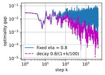
fixed eta = 0.8:     mean gap, last 1000 steps = 2.34e-02
fixed eta = 0.4:     mean gap, last 1000 steps = 1.08e-02
decay 0.8/(1+k/100): mean gap, last 1000 steps = 5.67e-04
Fixed \eta approaches a nonzero floor; 1/k continues toward zero: noise moves the rate class from geometric to polynomial.
Newton’s Method: Accuracy and Cost
Curvature as information
Newton minimizes the local quadratic exactly, \mathbf{x}_{k+1}=\mathbf{x}_k-(\nabla^2 f)^{-1}\nabla f. On a positive-definite quadratic, the exact-arithmetic step is affine-invariant and reaches the minimizer in one iteration. Quadratic convergence holds locally under a nonsingular, Lipschitz-continuous Hessian.
Newton on the quadratic: |x_1| = 0.0e+00 after one step
GD with the optimal step contracts by 0.9802 per step; it needs 691 steps for |x_k| <= 1e-6
Newton iteration 1:  |grad| = 2.8e-01
Newton iteration 2:  |grad| = 3.2e-02
Newton iteration 3:  |grad| = 1.1e-03
Newton iteration 4:  |grad| = 1.2e-06
Newton iteration 5:  |grad| = 1.6e-12
Newton iteration 6:  |grad| = 3.1e-17
agrees with the SGD section optimum: True
Dense arithmetic limits the method: storage is O(d^2) and a generic solve is O(d^3) per step. Large models therefore use Hessian–vector products, limited-memory secant approximations, or structured and diagonal preconditioners.
Step control and curvature determine the method
Wrap-up
- Steepest descent follows from Cauchy–Schwarz; finite progress also requires a sufficiently small step.
- L-smoothness gives the descent lemma and an O(1/K) stationarity bound without convexity.
- On quadratics GD decouples per mode: stability \eta<2/L, cost linear in \kappa.
- Convexity upgrades to global optimality; momentum turns \kappa\to\sqrt{\kappa}, optimal for first-order.
- SGD is unbiased with 1/b variance and has nonzero stationary error under a fixed step; suitable decay permits convergence under the stated assumptions.
- Newton ignores \kappa but costs O(d^3), hence its diagonal and low-rank stand-ins (Adam, L-BFGS).
Learning-rate analyses compare first-order decrease with curvature error, and gradient signal with stochastic noise.