Divergences and Distances Between Distributions

Dive into Deep Learning · §28.2

Comparing probability distributions
f-divergences, optimal transport, and the objective map.

Which notion of closeness?

Motivation

Every generative model minimizes “distance from model to data.” The choice of divergence fixes the objective, the gradients, and the failure modes. Three families:

f-divergences: a convex f of the ratio p/q,
integral probability metrics: the largest mean gap,
optimal transport: the cheapest way to move mass.

The f-divergence family

one convex generator, many divergences

The f-divergence template

The f-divergence

D_f(P\|Q) = \mathbb{E}_{x\sim Q}\bigl[f(p/q)\bigr] for convex f with f(1)=0.

Proof that D_f \ge 0: \mathbb{E}_Q[f(p/q)] \ge f(\mathbb{E}_Q[p/q]) = f(1) = 0. Jensen, once, for the whole family. \blacksquare

Convexity of f yields non-negativity.

Another application of Jensen gives data processing: pushing P and Q through any channel K only loses distinguishability, D_f(PK\,\|\,QK) \le D_f(P\|Q), for every f at once.

A gallery of generators

The gallery

One curve f per divergence:

KL: u\log u · reverse KL: -\log u
Pearson \chi^2: (u-1)^2
Hellinger: (\sqrt u-1)^2
total variation: \tfrac12|u-1|
Jensen–Shannon (symmetric)
\alpha-family: a parameter from reverse to forward KL; its log-transform is Rényi’s D_\alpha

Near P=Q all agree, \propto f''(1)\,\chi^2; they differ only far apart.

The gallery, numerically

The numbers

Each generator gives a different number on the same pair; KL is asymmetric, JS symmetric and capped below \log 2:

KL           D_f(P||Q) = 0.3961   D_f(Q||P) = 0.3653
reverse KL   D_f(P||Q) = 0.3653   D_f(Q||P) = 0.3961
chi^2        D_f(P||Q) = 1.0133   D_f(Q||P) = 0.8000
Hellinger^2  D_f(P||Q) = 0.1862   D_f(Q||P) = 0.1862
TV           D_f(P||Q) = 0.4000   D_f(Q||P) = 0.4000
JS           D_f(P||Q) = 0.0911   D_f(Q||P) = 0.0911
JS via the mixture formula: 0.0911

Duality: divergence as a game

the Fenchel conjugate, the f-GAN, and mode geometry

A divergence is a game against a critic

Variational form

A convex f is the envelope of its tangents, so for any critic T:

D_f(P\|Q) \ge \mathbb{E}_P[T] - \mathbb{E}_Q[f^*(T)],

expectations only, no densities. The ordinary GAN is the Jensen–Shannon case.

Tight only at the right critic

The f-GAN

For the \chi^2 generator the bound hits the true divergence exactly at the optimal critic T^\star = f'(p/q), and any other critic falls short:

exact chi^2(P||Q)           = 1.0133
bound at the optimal critic = 1.0133
bound at a perturbed critic (scale 0.5): 0.9678
bound at a perturbed critic (scale 1.0): 0.3661
bound at a perturbed critic (scale 2.0): 0.9600

An undertrained critic biases the estimate low; the adversary’s job is to make the bound tight.

Forward vs. reverse KL

Mode geometry

Same target, two optima: forward KL (maximum likelihood) must cover every mode; reverse KL (variational inference) concentrates on one, paying \log(1/0.7) nats for the mass it drops:

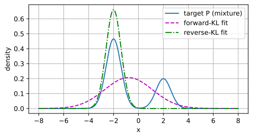
forward KL             mu = -0.800, sigma = 1.929, KL = 0.558 nats
reverse KL             mu = -1.998, sigma = 0.603, KL = 0.356 nats
reverse KL, 2nd start  mu = +1.995, sigma = 0.607, KL = 1.202 nats

Metrics: when densities fail

total variation, MMD, and optimal transport

Total variation and Pinsker

The strongest test

\mathrm{TV}(P,Q) = \sup_A|P(A)-Q(A)| = \tfrac12\|p-q\|_1. Hand a tester one sample: the best test succeeds with probability \tfrac12(1+\mathrm{TV}); in the cryptographers’ convention, an advantage of exactly \mathrm{TV}.

Pinsker: \mathrm{TV} \le \sqrt{D_{\mathrm{KL}}/2}, so a small KL bounds the distinguishing advantage of every event.

Pinsker’s constant is sharp

A stress test

Across ten thousand random pairs the ratio \mathrm{TV}/\sqrt{D_{\mathrm{KL}}/2} never exceeds 1, and near-fair coins push it to 0.999999:

max TV / sqrt(KL/2) over 10,000 random pairs: 0.9926
coins 1/2 vs 1/2+0.1: TV / sqrt(KL/2) = 0.989881
coins 1/2 vs 1/2+0.01: TV / sqrt(KL/2) = 0.999900
coins 1/2 vs 1/2+0.001: TV / sqrt(KL/2) = 0.999999

The factor \tfrac12 cannot be improved.

IPMs and the kernel trick

Sample-only

An integral probability metric is \sup_{f\in\mathcal F}\mathbb{E}_P[f]-\mathbb{E}_Q[f]. Over an RKHS ball it becomes MMD, a closed-form kernel expectation with no critic and no densities:

MMD^2, same distribution : +0.00054
MMD^2, mean shifted 0.5  : +0.05890

A half-\sigma shift jumps \mathrm{MMD}^2 by two orders of magnitude.

Optimal transport and Wasserstein

Moving mass

On disjoint supports every f-divergence is constant (zero gradient) while W_1 still moves smoothly. That is the WGAN.

Dual (Kantorovich–Rubinstein): the 1-Lipschitz critics. In one dimension, W_1 = \int|F_P - F_Q|.

One integral replaces a linear program

Wasserstein-1

The CDF formula and a 36-variable transport LP agree to ten digits:

W1 via the CDF formula : 1.7000000000
W1 via the primal LP   : 1.7000000000

Beyond one dimension no such formula exists, and the LP has n^2 variables.

Sinkhorn and entropic regularization

Entropic OT

Sinkhorn’s row/column rescalings solve the -\varepsilon H(\gamma)-regularized plan on a GPU. At \varepsilon=1 the diffuse plan costs 1.77 vs 1.70; decreasing \varepsilon approaches the LP’s monotone transport plan:

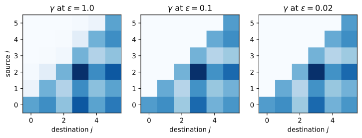
epsilon = 1.00: entropic cost = 1.7700   (unregularized LP: 1.7000)
epsilon = 0.10: entropic cost = 1.7000   (unregularized LP: 1.7000)
epsilon = 0.02: entropic cost = 1.7000   (unregularized LP: 1.7000)

Scores and the objective map

the normalizer-free divergence, and the unifying table

Scores Cancel Unknown Normalizing Constants

Fisher divergence

s_P(\mathbf x) = \nabla_{\mathbf x}\log p drops the intractable Z entirely, since \nabla\log Z = 0. The Fisher divergence compares score fields, the basis of score matching and diffusion.

Normalizer-blindness, numerically

The point

Rescaling the density leaves the score unchanged to floating-point precision, and the Gaussian Fisher divergence matches its closed form:

mixture score, max |analytic - numerical|: 3.52e-04
score change from rescaling p by 2.7    : 1.82e-12
Fisher divergence N(0,1)||N(1,1): quadrature 0.500000, closed form 0.500000

This is why score matching works where density estimation cannot.

Stein’s identity and goodness of fit

KSD

For any smooth f, \mathbb{E}_P[f' + f\,s_P] = 0: a fingerprint of P that needs only its score. A systematic population violation distinguishes the distributions; a finite-sample test still requires calibration:

rng = np.random.default_rng(7)
z = rng.standard_normal(1_000_000)
# Stein operator for P = N(0,1):  (A_P f)(x) = f'(x) - x f(x)
for name, f, fprime in [('x^3', lambda t: t ** 3, lambda t: 3 * t ** 2),
                        ('sin x', np.sin, np.cos)]:
    val = (fprime(z) - z * f(z)).mean()
    print(f"E[ f'(Z) - Z f(Z) ] for f(x) = {name}: {val:+.4f}")

E[ f'(Z) - Z f(Z) ] for f(x) = x^3: +0.0020
E[ f'(Z) - Z f(Z) ] for f(x) = sin x: +0.0005

The kernel Stein discrepancy turns this identity into a test statistic; its descent direction yields SVGD.

Divergences Induce Distinct Idealized Objectives

Objective comparison

MLE/flows → forward KL · VAE → reverse KL · optimal GAN critic → JS · f-GAN → an f-divergence · WGAN → W_1 · MMD-GAN → MMD · diffusion → Fisher · SVGD → KSD.

These correspondences describe population objectives under their idealized critic and model assumptions; finite optimization can behave differently.

Divergences Encode Different Modeling Priorities

Wrap-up

f-divergence = \mathbb{E}_Q[f(p/q)]; Jensen gives D_f \ge 0 and its DPI.
The \alpha/Rényi family sweeps reverse \to forward KL.
Fenchel duality turns any f into a critic game (the f-GAN); GAN is the JS case.
Forward KL tends to cover modes; reverse KL may concentrate on one.

TV is the best single-sample advantage; Pinsker bounds it by \sqrt{\mathrm{KL}/2}.
W_1 remains informative on disjoint supports (WGAN), though not necessarily smooth; Sinkhorn approaches the unregularized transport problem as regularization vanishes.
The score drops Z; the Fisher/Stein row powers diffusion and SVGD.

Next: mutual information, a divergence from independence, put to work in representation learning.